Category Archives: Excel

March Madness: Using Excel to Pick the Upset

Bracket Mania

It’s that time again! Time to get out the office pool and place all of your stock in one team to take you to the finals and earn you those much sought after office bragging rights. Last year, to aid in my bracket-making decision, I decided to write a way to be able to generate a randomized bracket for the NCAA college Men’s Basketball Tournament using Excel. This year, I dug a bit more into using an alternative method, the KenPom rating, to see if I could predict a better bracket. You can dig into this stuff endlessly (or so it seems), starting out with the source of the rankings at KenPom.com. KenPom.com is a college basketball statistics site that has been featured on FiveThirtyEight, Mediaite, and The Wall Street Journal for its predictions in game outcomes. Ken Pomeroy, the creator of the site, has statistics dating back to the 2003 season, and his research is used by many college basketball teams to gain a competitive advantage.

The bracket I made this year was built in a couple of different ways. First, I used the seed strategy, where a higher seed historically wins X% of the time. Second, I used KenPom to figure out how the match-ups might work based on a random outcome. This second method does allow for some very volatile outcomes, so use at your own risk!

I am attaching a project that goes into all of the details of generating the brackets, and I have updated it from last year to get the latest attempt to win some bragging rights.

Download the Brackets and Excel Spreadsheets

To see the completed Excel spreadsheet and my 2014 bracket picks, click the links below. May the odds be ever in your favor!

The full Excel file: NCAATournamentBracket
The C# project: TournamentBracket_2014
My tournament bracket: TournamentBracket_2014_Final

Note: To save the bracket, you need to turn off the auto-calculation feature. This is due to Excel always updating the RAND() output on each change. I recommend changing it to Manual Calculation, and using F9 to run it when you want new values. Don’t forget, this may eventually run through every possible outcome; let me know if you end up winning anything from this!

Predictions

And the final prediction for this year is: Arizona wins it all.

Yes, the likelihood of me being correct is small, but given the current odds (6 / 1), I am feeling pretty good about it. Which does, of course, guarantee that this will be the incorrect bet.

Editor’s Note: Chad (the author of this post) hails from Arizona, so fair warning, there may be some home-state bias in this post.

How to Sort Locked Cells in Protected Worksheets

Problem

When creating workbooks with protected sheets, it is common to want to allow users to get different views of the data by sorting and filtering,  without allowing them to change the data. However, while filtering works fine on locked cells, sorting does not. Even if Sort is enabled in the worksheet protection settings, if a user attempts to sort locked cells when a worksheet is protected, Excel throws the error “the cell or chart you are trying to change is protected and therefore read-only.” There is no obvious way to allow users to sort data on a protected worksheet.

Details

Locked VS. Unlocked Cells in Excel

The purpose of locking a cell is to prevent a user from editing the content of a cell when a worksheet is protected. This means when worksheet protection is turned off, a locked cell is no different from an unlocked cell. By default, all cells in an Excel worksheet are locked.

In order to unlock cells in Excel:

  1. Unprotect the sheet you are working on
  2. Right-click the cell, select “Format Cells”
  3. Select the “Protections” tab
  4. Uncheck the “Locked” checkbox property
  5. Click “OK”

Lock Cells Dialog

Lock Cells Dialog Box

It is also possible to unlock specific ranges of cells in Excel using the Allow Users to Edit Ranges feature in the Review tab. Making ranges editable for ranges of cells makes the cells behave like unlocked cells for the most part (e.g. their content is editable). However, the cell’s official locked/unlocked status does not actually change. See this Microsoft Excel article  for more details about how to unlock ranges of cells.


About Worksheet Protection Properties

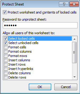
When you protect a sheet, Excel allows you to select from 15 different permissions you want to give to all viewers of the worksheet. You can allow users of the worksheet to:

  • Select Locked Cells
  • Select Unlocked Cells
  • Format Cells
  • Format Columns
  • Format Rows
  • Insert Columns
  • Insert Rows
  • Insert Hyperlinks
  • Delete Columns
  • Delete Rows
  • Sort
  • Use Autofilter
  • Use PivotTable Reports
  • Edit Objects
  • Edit Scenarios

Protect Sheet Dialog

properties

How Protection Properties are Affected By Locked Cells

When a cell is locked, not all worksheet protection properties operate as you’d expect. Four of the properties do not work when a cell is locked:

  • AllowSort
  • AllowDeleteColumns
  • AllowDeleteRows
  • AllowInsertHyperlinks

This is because in order to use these features the affected cell’s content must be changed. For example, using “Sort” does not just change the order of how the cells are viewed, it actually changes the values of the cells so that they are sorted. Due to this implementation of “Sort,” this worksheet protection property does not work when the cells are locked.

Solution

There are two approaches we can take to solve this issue:

Solution 1: Using “Allow Users to Edit Ranges” to Allow Locked Cell Sorting (RECOMMENDED)

This solution takes advantage of how allowing users to edit ranges makes locked cells behave like unlocked cells.

Step 1: Make cells editable so that sorting will work.

Add cells we want to sort to a range and make that range editable in “Allow Users to Edit Ranges.” This allows users to edit these cells when the worksheet is protected, even if they are locked cells.

  1. Select all the cells you would like the user to be able to sort, including their column headings.
  2. Go to the Data tab and click Filter. An arrow should appear next to each column header.
  3. Go to Review tab-> Allow Users to Edit Ranges
    1. Click “New…”
    2. Give the range a title.
    3. “Refers to Cells” should already contain the cells you want to allowing sorting on.
    4. If you want to allow only certain people to sort, give the range a password.
    5. Click “OK”

Step 2: Prevent users from editing these cells

When protecting the worksheet, uncheck “Select Locked Cells” worksheet protection property. This will prevent users from editing the cells.

  1. In the “Allow Users to Edit Ranges” dialog:
    1. Click “Protect Sheet…”
    2. Give the worksheet a password
    3. Uncheck the worksheet protection property called “Select Locked Cells”
    4. Check the “Sort” property and the “AutoFilter” properties
    5. Click “OK”

This solution allows users to use the Auto Filter arrows in the column names or the Sort buttons in the Data tab to sort data. Another benefit is that you have the option of allowing only certain users to sort by giving the range a password. Please note that this range password is separate from the password you set to protect the sheet.

Solution 2: Using Macros to Allow Locked Cell Sorting

To use a Macro to allowed the sorting of locked cells, you will need to make a macro for every sort operation you would like to allow. For example, ascending sorts and descending sorts would have to be written in separate macros. In addition, not all users have macros enabled because they are a security risk. However, the advantage of macros is that you don’t need to configure your template in any special way.

The macro we will write unprotects the sheet, selects a range called “range1,” sorts range1, and protects the sheet again:

Sub Macro1() 
' 
' Macro1 Macro 
' 
' Keyboard Shortcut: Ctrl+d 
'    
     //unprotect sheet 
     ActiveSheet.Unprotect
     //selects range     
     Application.Goto Reference:="range1"     
     //clears sort
     ActiveWorkbook.Worksheets("Sheet1").Sort.SortFields.Clear     
     //does descending sort, sets sort properties 
     ActiveWorkbook.Worksheets("Sheet1").Sort.SortFields.Add Key:=Range("A1"), _
         SortOn:=xlSortOnValues, Order:=xlDescending, DataOption:=xlSortNormal
With ActiveWorkbook.Worksheets("Sheet1").Sort
         .SetRange Range("A1:A4")
         .Header = xlNo
         .MatchCase = False
         .Orientation = xlTopToBottom
         .SortMethod = xlPinYin
         .Apply
     End With
     //protects the work sheet again
     ActiveSheet.Protect DrawingObjects:=False, Contents:=True, Scenarios:= _
         False
 End Sub

New Webinar! Make Reports that Measure Up

Take a look at how OfficeWriter can turn your drab Excel reports into chart-topping spreadsheets. This month, it’s all about music as we cover your favorite bands, artists, and labels.

In this webinar we’ll cover:

  • Grouping and nesting in Excel
  • Using SQL Server Reporting Services (SSRS)
  • Charting in Excel and relationships between genre, artists, labels, and album price

When: Friday, August 23, 2013 at 1 P.M. EST

*Register early as space is limited.

Can’t attend? Register anyway, and we’ll send a copy of the slides and recording following the webinar.


Carpe Datum: How to Export Your GMail to Excel

Credit: Hongkiat.com

[Crossposted from Riparian Data]

Straightforward title, straightforward goal, ugly and roundabout (but free!) method of achieving it.

For some time now, I’ve had this goal: download my gmail data, analyze it, and visualize it.

The last time I tried this, I glossed over the whole getting your gmail data into Excel part. This is because I wasn’t able to do all of it myself–Jim had to take my ugly mbox data and make it Excel-readable.

But now, thanks to the basic python skills acquired in my data science class, I can do everything myself! Kinda. The code in part 3 will probably make a real programmer scream, but for the most part, it works–though it’s not fond of commas in subject lines. And if you, like me, are not a programmer–don’t worry! You can still run the code, using my trusty copy/paste/pray methodology.

Alors, here goes:

Step 1: From Gmail to Apple Mail

You have Apple mail, right?  You can also do this with Outlook, and probably other desktop clients.

1) In your Gmail settings, go to the “Forwarding and POP/IMAP tab” and make sure POP is enabled.

2) Now, add your Gmail account to your desktop client o’choice. If it’s already there, add it again–you’re going to be removing this one.

Important: Do not check the “remove copy from server after retrieving a message” box!

Step 2: From Apple Mail to mbox

This part is easy. Just select your mailbox in the desktop client, and go to Mailbox->Export Mailbox, and choose a destination folder.

Step 3: From mbox to csv

If you try to save your pristine mbox file as a csv, you will get a one column csv. Don’t do that. Instead, use these python scripts (also up on github).

The first script opens a blank csv file, and fills it with the subject, from, and date lines for each message in your mbox. I called it mbox_parser.py.

import mailbox import csv
writer = csv.writer(open("clean_mail.csv", "wb")) for message in mailbox.mbox('your_mbox_name'):     writer.writerow([message['subject'], message['from'], message['date']])

If you don’t know what python is, you can still run this script. Here’s how:

1) copy the above code to a plain text file, and save it as mbox_parser.py. Save it to the same folder you saved your mbox file to.

2) open your terminal (spotlight–>terminal)

3) type cd Users/your_account_name/directory_where_you_saved_your_mbox,

4) type  python mbox_parser.py

5) Voila! In your directory, you should see a new file, cleaner.csv.

You’ll notice that the ‘date’ column is a long, jam-packed date string. It’ll be much easier to Continue reading Carpe Datum: How to Export Your GMail to Excel

When to use SUMIF vs. Pivot Tables in Excel

SUMIF and PivotTables can both summarize data based on specific criteria, but they do so in completely different ways. In most cases, PivotTables are going to be faster and easier to get the data that you want, but sometimes using Excel formulas is the only way to handle complicated data.

All the examples from this blog post can be found in this workbook: SUMIF_PivotTable

WHY PIVOT TABLES ARE BETTER

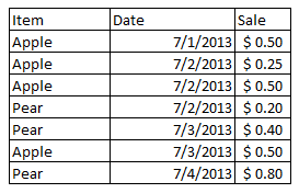
Let’s take a look at a quick example of some fruit sales data, where we want to find information like: all sales for a date, total sales for a fruit in the given time period, or total sales for a type of fruit on a given day.

ExampleData

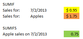
With SUMIF, you can specify the range of values you are using as the criteria (dates or fruit), the values you want to sum (sales), and the actual criteria that will determine if the values are included in the sum (“7/2/2013”, “Apple”). SUMIFS (new in Excel 2007) extends this functionality to allow multiple criteria (dates and fruit):

ExampleFormulas

Note: Excel also offers COUNTIF, COUNTIFS, AVERAGEIF and AVERAGEIFS starting in Excel 2007.

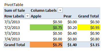
You can do the same with PivotTables, but the PivotTable will also handle sorting, grouping and organizing your data so you can just lift the aggregated values right out from the table:

ExamplePivotTable

Here the values are automatically generated by the PivotTable. No extra work needed aside from creating the PivotTable, which is as easy as selecting the data range and specifying where the table needs to go.

Excel also applies PivotTable styles, which change be switched in one click and you can even create your own custom styles.

WHY WOULDN’T YOU USE PIVOT TABLES?

I extended my fruit example to use sample data from the AdventureWorks database, where I wanted to compare online and retail sales for North America, broken down by quarter: Continue reading When to use SUMIF vs. Pivot Tables in Excel

Baseball’s All-Star Break: Predicting the Game Using Excel

Major League Baseball
Credit: Ampsportsduo.blogspot.com

In keeping with my sports theme from March, on March Madness and predicting the NCAA tournament, it is time to look at this season’s sport: Baseball. As you might know, Major League Baseball’s All-Star game is tonight, so let’s use Excel to pick which league (the AL or NL) will be victorious, so we can kick back and enjoy the game.

Baseball has long been associated with using stats to predict outcomes and player performances. This was made famous in the movie Moneyball, and has its own cottage industry around helping fantasy baseball players perform better. There is no shortage of information that can be gathered about baseball, with the whole industry even having deemed the term: sabermetrics.

Before jumping into the vastness of data, however, I want to point out where we are getting the data from. There are many different sources for baseball stats, many requiring a fee, but I will be referring to the Sean Lahman Baseball Stats Database. It is open source, so you can just download a version that works for you, and run with it. I am only going to look at the players who have actually appeared in the All-Star game and their year’s performance.

The other source of data is the year-to-date stats for the All-Star players. These can be gathered from the many, many sports sites (like ESPN.com), but is a manual process. I will leave it as an exercise for the reader to copy and paste those! You can find the sum of those in the example file attached.

Just to simplify things, we are going to use the old standbys: Earned Run Averages (ERA) and Batting Averages (BA) to compare the two Major League Baseball leagues. The other consideration is to analyze data from just the “Long Ball Era,” which started in 1994. Since the sport has been around so very long, it helps to categorize the data so you get a better apples-to-apples comparison.

The first step is to get the data into your database. I used the Access file download, since SQL Server 2008 R2 can import that directly, and you don’t have to do any of the conversions. The data is also available in CSV and MySQL format. Now that we have a nice almost relational database, all we need are a couple of SQL statements to get the data for our processing needs. (They have been attached for reference.)

On to building our Excel workbook. Continue reading Baseball’s All-Star Break: Predicting the Game Using Excel

ExcelTemplate: How to format alternating row colors

Problem

A common way to display data in Excel is to alternate the background color of every other row when displaying a large table of data. With ExcelWriter there are multiple ways to accomplish this. This post covers some possible ways to apply alternating row colors with ExcelTemplate.

There is another post that discusses how to do this with ExcelApplication.

Solution

Option 1: Format as Table in Excel 2007/2010

Starting in Excel 2007, Excel provides pre-formatted table styles which already contain alternating row or column colors. This is the easiest way to format your data with alternating row colors. Note: these table styles may not render properly in Excel 2003 or in the XLS file format.

To format an area of cells as a table:

1. Highlight the area of cells.

2. Go to Format as Table in the ribbon.

3. Select a table style from the available styles.

4. If you chose to include your table header row, make sure to check off “My table has headers” in the confirmation dialog.

There are basic options for modifying the banding patterns:

You can also create new table styles:

You can do this for ExcelTemplate templates:

When the rows of data are inserted, the color banding will be applied:

Option 2: Use Conditional Formatting

The other approach is to use conditional formatting in the template to achieve alternating row colors. This may be more appropriate if you are not certain if your end-users will have Excel 2007/2010.

1. Create an ExcelWriter template with data markers in Excel.

2. Highlight the cells with data markers that correspond to the data you wish to display with alternating background colors.

3. From the menu, choose Format>Conditional Formatting. The formatting you define for this row will be applied to every new row that will be inserted by ExcelTemplate at runtime.

4. First define the formatting for even rows. In the “Condition1” field, choose “Formula Is” and in the formula field, type the following formula:

 =MOD(ROW(),2) = 0 

This formula uses the MOD( ) function to determine if the number of the current row (returned by the ROW( ) function) can be evenly divided by 2.

5. Click on the “format” button.

6. Click on the “patterns” tab and select a background color.

7. Now set a condition for odd rows, by clicking “ADD” and following the same steps as above but with a different formula:

 =MOD(ROW(),2) = 1 

8. Save the template and use it in your ExcelWriter application.

When ExcelTemplate imports new rows of data, the conditional formatting will also be applied to all the new rows:

How to Download Files Containing Special or Non-ASCII Characters in the Filename Using ASP.NET

Credit: http://lifehacker.com/5690522/how-to-enable-non+ascii-characters-on-linuxA couple months ago, I worked with file downloads that had filenames with non-ASCII Unicode characters, as well as special characters, such as semi-colons, commas, periods, and others (@, %, +, {, }, [, ], $, #, &, =). Here is an example of a filename that has all of those characters:  日本人 中國的 ~=[]()%+{}@;’#!$_&-  éè  ;∞¥₤€   .txt    

After a couple days of online research,  I finally found a solution that worked across different major browsers like IE8, IE9 and IE10, Firefox 21, Chrome 27, Safari 5 (on Windows). These are the most up-to-date versions as of this writing. Opera mostly works fine as well; however, I noticed that it doesn’t like the space and curly bracket characters.

Without going into detail about character encodings in the HTTP headers, I’d like to mention two major pieces of information you should know that I found regarding this issue:

1. According to the section 2.3 in RFC-2183 (Content-Disposition header field), the “filename” parameter in the Content-Disposition header can only use the US-ASCII characters.

2. However, as specified by RFC-5987 and RFC-2231, the correct encoding can be included right in the header field by using the filename* syntax and then by percent-encoding the non-ASCII characters in the filename. For example, for the filename “test-€.txt,” the content-disposition header would look like the following:  attachment; filename*=utf-8”test-%E2%82%AC.txt. Here is the .NET code that I had for writing the response header:

Response.AddHeader(“Content-Disposition”, “attachment; filename*=utf-8”” + Server.UrlEncode(fileName);

However, when I tried that syntax with my test filename Continue reading How to Download Files Containing Special or Non-ASCII Characters in the Filename Using ASP.NET

How to open a report from SQL Server Reporting Services with the Application object

Problem

You want to modify your reports with the WordApplication or ExcelApplication object after they’ve been populated with data by SQL Server Reporting Services. The ExcelApplication or WordApplication object’s Open method can’t pull a report from a report server, so how do you open a SSRS report with OfficeWriter?

Solution

For simplicity and ease of reading the code examples and text in this article refer to the ExcelApplication object exclusively. However, the exact same techniques can be used with the WordApplication object. The only strict requirement for opening reports from SSRS is for the Open method to have an overload that takes a Stream argument, which both objects have.

SQL Server Reporting Services exposes a web service that lets programs access and work with the reports on the server. The web service has a number of functions for interacting with a report server and in fact is the same API that the Report Manager tool is built on top of. One of its functions will let us retrieve a fully rendered report that we can then pass to the ExcelApplication object. Once the ExcelApplication object has opened the report, it can be used as if it were any other file.

Getting a Reference to the Report Server

There are a number of different ways to access a report server to manage your reports. The MSDN documentation has detailed instructions for all the different techniques. The most powerful way, and the one that the Report Manager application uses, is to use the report server’s web service, or SOAP API. The easiest way to use the web service is to add the report server as a web reference in Visual Studio. This will allow us to make web service calls to the report server as though it were any other object in a .NET project. I’ll provide a brief overview of the steps to add a report server as a web reference; details can be found at MSDN. Continue reading How to open a report from SQL Server Reporting Services with the Application object

Workbook colors are not displayed as expected in older versions of Excel

Problem

When using ExcelWriter’s ExcelApplication object to generate a new workbook, custom colors that are assigned in code to fonts, charts, cell backgrounds, etc., display incorrectly on the client when the workbook is generated.

OR

When creating an Excel File or an Excel file to use as a template with the ExcelTemplate object using Excel 2007 and above, colors are not colors are not preserved in Excel 2003 or older.

Continue reading Workbook colors are not displayed as expected in older versions of Excel