All posts by Alison

Full time OfficeWriter Product Owner, part-time pivot table enthusiast.

What’s New in OfficeWriter 9

OfficeWriter version 9 is now available! Here is a breakdown of what you can find in the latest version of OfficeWriter.

Calculation Engine

OfficeWriter version 9 kicks off with the initial release of the calculation engine for ExcelWriter. Now you can evaluate the formulas in your XLSX and XLSM files before delivering spreadsheets. Applications that can’t evaluate formulas, such as mobile apps, Outlook preview, or Excel in protected view, will show the updated values when workbooks are opened. You can also use the calculation engine to update formulas before reading them with ExcelApplication.

Currently, the calculation engine supports evaluating all of the formulas in a given workbook through the method Workbook.CalculateFormulas. This will update all the cell values based on the formulas. Check out our list of the formulas that the calculation engine supports.  If there’s a formula you need that we don’t have yet, contact our support team to submit a request!

PowerPointWriter

v9Blog5

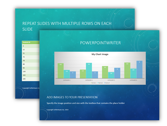
The PowerPointWriter beta program has been going strong, and we’re excited for the official release. PowerPointWriter introduces a template-based approach to generating PowerPoint presentations (PPTX) dynamically.  Taking the best principles from ExcelWriter and WordWriter, PowerPointWriter is flexible and easy to learn.

Learn more about what PowerPointWriter can do for you with our Features overview,  use cases, and API Introduction and Tutorials.

New Excel Features

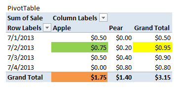
Pivot tables from multiple data sources

In OfficeWriter version 8.2, the PivotTable API for ExcelApplication was added to ExcelWriter. In OfficeWriter version 9 you can build multiple consolidation range pivot tables.  These pivot tables are created from multiple consolidation ranges and automatically generate pivot fields using the data. We have a short video to help explain how these special pivot tables work: [5 minutes with Chris – PivotTables]

v9Blog3

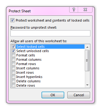
WORKSHEET PROTECTION PROPERTIES

ExcelWriter now offers the same protection options as Excel that change how a worksheet is locked down when it’s protected. Set SheetProtection properties to customize what users can interact with after Worksheet.Protect is called.  Check out our knowledge base article for more on how to use this new feature!

Binding custom objects to Excel

In OfficeWriter version 9 ExcelTemplate supports the ability to bind lists of custom objects to templates.  For example, you have some custom Order objects that contain information about OrderID, DeliveryDate, PurchaseAmount, and CustomerID. These Order objects are in a list called ListOfOrders.

In your template, you can reference the object properties in the data marker: %%=ListOfOrders.OrderID. ExcelWriter will treat each object in the list as though it were a row of data in a table.

For more information about how ExcelWriter imports data, please visit our documentation: ExcelWriter Basic Tutorials.

And more!

For more information about additional information about all of the changes in OfficeWriter, see our Change Log.

How to Format Rows or Columns only if they Contain Values

Problem

You want to apply particular styles or formats, but only to rows or columns that actually contain values. Here are some examples of styles and formats that you might want to apply to specific rows or columns:

  • Background/Foreground colors
  • Borders
  • Fonts
  • Text orientation, justification, indentation, orientation, number format
  • Horizontal/vertical alignment
  • Cell locked/unlocked when worksheet is protected

Notes:

Conditional formatting is useful if you wish to apply particular formatting that changes depending on the actual values in the cells. Go to Conditional formatting resources.

A similar technique can be used to format just an area. For specifics, see Format an area instead of rows or columns.

Solution

This solution has several steps:

  1. Define an area that contains the populated cells in order to determine which rows and columns to format.
  2. Create the style to apply.
  3. Loop through the rows or columns in the area and apply the style to each row or column.

Step 1:

Get the populate cells in the worksheet. There are two ways to do this:

A. Worksheet.Populated Cells – 

Use Worksheet.PopulatedCells to return an area of all the cells that are populated starting with the top left cell that contains a value or formatting, down to the bottom right cells. It includes both cells with values/formulas as well as cells that contain formatting (e.g. background color, conditional format etc.)

ExcelApplication xla = new ExcelApplication();
Workbook wb = xla.Open("MyUnformattedWB.xlsx");
Worksheet ws = wb.Worksheets["SheetToFormat"];
 
Area populatedArea = ws.PopulatedCells;


B. Use a named range

Add a named range in the template file around the area that will contain the populated cells and then use Worksheet.GetNamedRange(String) or Workbook.GetNamedRange(String) to retrieve the named range. Use Range.Areas to get a handle on the desired area.

This is less expensive than Worksheet.PopulatedCells since ExcelWriter does not need to go through the worksheet to figure out which cells contain values.  There are some limitations to this approach:

  • The number of columns in the named range will not change after data is imported. If there are columns in the populated named range that do not contain data, the named range won’t reflect that.
  • The number of rows in the named range will only change after data is imported if  the named range is wrapped around ExcelTemplate data markers and new rows are inserted.
  • If you are using Worksheet.ImportData, the named range will not update to reflect where the live data is.
ExcelApplication xla = new ExcelApplication();
Workbook wb = xla.Open("MyUnformattedWB.xlsx");
Range myRange = wb.GetNamedRange("AreaWithValues");
 
Area populatedArea = myRange.Areas[0];

Step 2:

Create the desired Style with Workbook.CreateStyle().

For this example, we want to leave the populated cells unlocked, but leave the rest of the cells locked when the worksheet is protected. This is done by setting Style.CellLocked.

Style unlockStyle = wb.CreateStyle();
unlockStyle.CellLocked = false;

Step 3:

Determine the first row/column in the area with Area.FirstColumn or Area.FirstRow. Get the total number of rows/columns in the populated area with Area.RowCount or Area.ColumnCount.

int colStart = populatedArea.FirstColumn;
int totalCol = populatedArea.ColumnCount;

Step 4:

Iterate through the rows/columns with Worksheet.GetColumnProperties(int) or Worksheet.GetRowProperties(int). Call ApplyStyle on the appropriate RowProperties or ColumnProperties with ColumnProperties.ApplyStyle(Style) or RowProperties.ApplyStyle(Style). Applying the style on an entire row or column will consume less memory than applying the styles to individual cells.

for(int i = colStart; i < totalCol; i++)
{
     ws.GetColumnProperties(i).ApplyStyle(unlockStyle);
}
 
//For worksheet protection, we also need to protect the worksheet
ws.Protect("MyPassword");

Additional References:

Applying Formatting to just an Area instead of Rows or Columns

If you want to apply the formatting just to specific cells, you can use Area.ApplyStyle()  or Area.SetStyle() instead of looping through the area to apply the style to each row or column.

IMPORTANT: This is only recommended for small areas.  Area.ApplyStyle and Area.SetStyle apply the style to each cell within the area, which increases the time and memory needed to process the file.  Applying styles on a per-row or per-column basis is the recommended best practice since the style is applied to the RowProperties or ColumnProperties object, instead to each individual cell.

Conditional Formatting

Charts not rendering correctly when viewed in non-Excel applications

Problem

An ExcelWriter-generated file with charts displays correctly when opened in Excel.  When the same file is opened in an application that does not have the full Excel functionality, such as Outlook preview or in a mobile application, the charts are missing data or have the wrong data.

When a workbook is opened in Excel, all of the cell values are updated based on the current state of the file. Excel caches these most recent cell values and writes them out to the file. Many mobile apps or applications with a “preview” functionality where the file is locked from being updated, do not have the ability to recalculate the cell values and rely on those cached values to render the charts. When the cached values are not available, the charts may be rendered incorrectly so they may appear to have no data, wrong data, or may not appear in the file at all.

Below are common scenarios where the workbook cannot be fully updated:

  • Mobile applications
  • Applications with “preview,” such as Outlook’s attachment preview
  • Excel’s protected mode, which is activated when files are downloaded from the internet and opened in Excel before saving to disk

Starting in v8.3, ExcelWriter writes out the cached cell values to integrate better with applications that don’t have the ability to update the workbook. However, there are still some limitations that prevent charts from being rendered correctly. This article describes the limitations and expected behavior of rendering charts in files that were generated in ExcelWriter v8.3 or later. 

If you are experiencing issues

Jump to:

Details

iOS Applications

Charts are missing – Certain charts are not supported by iOS, regardless of whether they are in files generated by Excel, ExcelWriter, or some other application. An example of this is the bubble chart. These charts may not be rendered at all, depending on the application. More information is available in this article: Charts in ExcelWriter files are missing when viewed on iOS devices.

Charts are visible, but incorrect – If the chart is visible, but the data appears to be incorrect, then the chart may have data that contains formulas, formatted numbers, or it may be a PivotChart (see below for more info).

Chart data contains formulas

As of v9.0, ExcelWriter has the ability to calculate formulas with the Workbook.CalculateFormulas method. However, for the initial release, only a limited number of formulas are supported.

If ExcelWriter is unable to evaluate formulas (i.e. the formulas you are using are not yet supported or you are using a version prior to v9.0), or Workbook.CalculateFormulas is not called, then the most up-to-date values will not be available. Instead, if there is a formula in the cell, we will write a “0” to the cached chart field. Despite not being an accurate value, having the cached value reduces the risk of the chart not being rendered or the the application from crashing due to the missing data.

Chart data contains values with number formats applied

ExcelWriter does not have the ability to render numbers based on number formats (e.g. percentage). In the case that a number has a number format applied, the underlying value will be used for the cached field. For example, 6.5% has actual numerical value 0.065, which is the value that ExcelWriter will write to the cached field. This also applies to dates, which are stored as serial numbers in the file and then Excel uses the number format to render the formatted date. For more information about dates in Excel, please see this article: http://www.cpearson.com/excel/datetime.htm.

PivotCharts

PivotCharts have a different structure than regular charts and depend on the entire PivotCache being refreshed to be updated.  Updating the PivotCache is an operation that must be performed in Excel or an application that has the ability to do so. ExcelWriter does not have the ability to refresh the PivotCache and update the PivotCharts. The file will need to be opened in Excel (not in protected mode) in order to update the PivotCache.

Charts in ExcelWriter files are missing when viewed on iOS devices

Problem

An ExcelWriter-generated file with charts displays correctly when opened in Excel, but when the same file is opened on an iPad or iPhone, the charts are missing from the file. There are two causes for this behavior:

  1. The chart type is not supported by iOS. – Some chart types are not supported in iOS and will never appear when viewed on an iPad or iPhone, regardless of whether the file was created in Excel or ExcelWriter. An example of this is the “bubble chart.” This is an issue with iOS mobile applications – not ExcelWriter.
  2. Charts in files generated by ExcelWriter v8.2 and earlier are not visible when viewed on iOS devices. – These chart types are supported in iOS and appear correctly on iPads or iPhones when the charts were created in Excel. If the file was generated by ExcelWriter, the charts are missing when viewed on iOS mobile devices. This is a known issue and was resolved in OfficeWriter 8.3.

This article describes why the second scenario occurs and the expected behavior when viewing charts created by OfficeWriter 8.3 or later.

Solution

When a workbook is opened in Excel, all of the cell values are updated based on the current state of the file. Excel caches these most recent cell values and writes them out to the file. Many mobile apps or applications with a “preview” functionality where the file is locked from being updated, do not have the ability to recalculate the cell values and rely on those cached values to render the rest of the file, including charts.

For iOS devices specifically, if the cached cell values are not available, most applications will not render the charts at all. ExcelWriter was not writing out cached values for the cells. Starting in OfficeWriter 8.3, ExcelWriter will copy the cell values to the cached field. This allows iOS applications to render the charts.

Limitations of Rendering Charts

In certain cases, the charts will be visible but may not look as expected. This is due to limitations in ExcelWriter’s ability to write out the cached values. For more information, please see Charts in ExcelWriter files not rendering correctly outside of Excel.

What’s New in OfficeWriter 8.6

64-bit Support in OfficeWriter Designer

OfficeWriter 8.6 marks the initial release of the OfficeWriter Designer .NET, a redesign of the original OfficeWriter Designer, using the latest technologies and best practices.

DesignerdotNetRibbon

The OfficeWriter Designer .NET is available for both 64-bit and 32-bit Excel and includes:

  • Better user experience with updated dialog boxes
  • Improved access to Report Properties
  • Stronger support for viewing reports with parameters
  • New import template functionality (also available in the original OfficeWriter Designer)

DesignerDotNetNewDialogs

The Designer .NET does not currently have full backwards compatibility with the original OfficeWriter designer. To find out if the Designer .NET will support your reports, review our quick guide or read about all of the differences in full in our documentation.

The OfficeWriter Designer .NET is available for download from our product updates page or through our evaluation sign-up.

Classic Pivot Tables

Starting in OfficeWriter 8.6, you can create PivotTables with the classic grid layout using the PivotTableSettings.ClassLayout property. This is the same as setting the classic layout property under PivotTable options. Continue reading What’s New in OfficeWriter 8.6

When to use SUMIF vs. Pivot Tables in Excel

SUMIF and PivotTables can both summarize data based on specific criteria, but they do so in completely different ways. In most cases, PivotTables are going to be faster and easier to get the data that you want, but sometimes using Excel formulas is the only way to handle complicated data.

All the examples from this blog post can be found in this workbook: SUMIF_PivotTable

WHY PIVOT TABLES ARE BETTER

Let’s take a look at a quick example of some fruit sales data, where we want to find information like: all sales for a date, total sales for a fruit in the given time period, or total sales for a type of fruit on a given day.

ExampleData

With SUMIF, you can specify the range of values you are using as the criteria (dates or fruit), the values you want to sum (sales), and the actual criteria that will determine if the values are included in the sum (“7/2/2013”, “Apple”). SUMIFS (new in Excel 2007) extends this functionality to allow multiple criteria (dates and fruit):

ExampleFormulas

Note: Excel also offers COUNTIF, COUNTIFS, AVERAGEIF and AVERAGEIFS starting in Excel 2007.

You can do the same with PivotTables, but the PivotTable will also handle sorting, grouping and organizing your data so you can just lift the aggregated values right out from the table:

ExamplePivotTable

Here the values are automatically generated by the PivotTable. No extra work needed aside from creating the PivotTable, which is as easy as selecting the data range and specifying where the table needs to go.

Excel also applies PivotTable styles, which change be switched in one click and you can even create your own custom styles.

WHY WOULDN’T YOU USE PIVOT TABLES?

I extended my fruit example to use sample data from the AdventureWorks database, where I wanted to compare online and retail sales for North America, broken down by quarter: Continue reading When to use SUMIF vs. Pivot Tables in Excel

How to create stock charts using ExcelApplication

Problem

You need to create stock charts like the High-Low-Close or candlestick charts that Excel provides, but ExcelApplication does not have an enumeration for these charts.

Solution

Introduction to Stock Charts

Excel can create four kinds of charts intended for analyzing stock data. These are often referred to as high-low-close or candlestick charts because of their distinctive shape. These charts can be easily created with the Chart Wizard in Excel.

It is possible to use these charts with ExcelTemplate as you would any other chart. While ExcelApplication contains enumerations for many kinds of charts it does not have one for stock charts. Because of this, they cannot be created directly. In this article I’ll explain how to use a line chart and some special formatting to create charts that look exactly like each type of stock chart provided by Excel.

Setting up the data

Stock charts require very specific data in a very specific order. If you look at the names of the charts in Excel, you’ll note that each of them is actually a list of the data that chart needs, in the order that chart needs it. The four kinds of charts are High-Low-Close, High-Low-Open-Close, Volume-High-Low-Close and Volume-High-Low-Open-Close. As you can see, there is significant overlap and the data always appears in the same order; only the presence or absence of Volume and Open Data is different. For all of the following examples, we’ll use the same data pictured below:

For simplicity, we’ll create areas for each section of data and name them volumeAreaopenAreahighArealowArea and closeArea. Now that we have that, we can start creating stock charts.

A Basic High-Low-Close Chart

The simplest chart to create is a High-Low-Close chart. This chart displays the high and low values for a stock as a vertical line, with a tick mark at the point where the stock closed for the day. To begin creating this chart, we’ll follow a formula that will remain the same for all of the other stock charts.

First, create Continue reading How to create stock charts using ExcelApplication

How to prevent line breaks after an empty merge field

Problem

When you use the WordTemplate object to populate a WordWriter template document with data retrieved from a data source, you may have situations in which a merge field is not bound to a value. The most common scenario is creating a mailing address. Each field of a mailing address may be represented by a merge field. Typically, the second line of the address is optional. In the generated document, if the merge field corresponding to the second line of the address does not have a value, a blank line may be present.

In Microsoft Word, a blank line generated during a mail merge can be suppressed using application settings. With WordWriter, a blank line is not automatically removed.

WordWriter template document:

Generated document:

Solution

The following discussion uses a merge field called AddressLine2 as an example, but is applicable to any field with optional value.

In the WordWriter template document, if the line break is separate from the AddressLine2 merge field, the line break will be present in the generated document whether or not Continue reading How to prevent line breaks after an empty merge field

How to create a drill-down report in Excel with hyperlinks

Problem

Reporting Services provides drill-down report behavior, where clicking on a populated data field generates another report based on the value of the data field clicked. This post addresses how to acheive similar behavior within Excel with OfficeWriter using Reporting Sevices URL access and Excel’s HYPERLINK function.

Solution

Overview

When the OfficeWriter renderer populates the Excel report with data, it inserts new rows for each row of data. This means that all Excel formulas are updated, including the HYPERLINK function formula. This approach uses this formula update functionality and imported data values to dynamically create hyperlinks that point to the Reporting Services URLs.

For the sake of example, “SalesReport” is the original report that contains a list of invoice IDs. “InvoiceReport” is the linked report that takes an InvoiceID as a parameter.

Reporting Services URL Access

Typically, Reporting Service reports are rendered through an application, such as the Report Manager. Reporting Services also allows for rendering reports using just URLs. The basic syntax to render a report wtith a parameter is:

 http://[servername]/reportserver?/[File path to report on Report Server] &rs:Command=Render&rs:Format=[Rendering Format]&[ParamID]=[Param Value] 

The URL for rendering the “InvoiceReport” in the OfficeWriter for Excel format, with Invoice ID 12345, is as follows:

 http://myservername/reportserver?/ InvoiceReport&rs:Command=Render&rs:Format=XLTemplate&InvoiceID=12345 

Notes:

How to create a custom SQL Server Reporting Services error page

Problem

When SQL Server Reporting Services (SSRS) encounters an error, it returns an error message which is displayed by Report Manager. The error message can include technical details that reveal more information than necessary or are potentially confusing or intimidating to a user. One example is the scenario in which the user attempts to export a report from Report Manager using the “Excel designed by OfficeWriter” option, but the report is not created using the OfficeWriter Designer. In this case, SSRS would return the following error:

 Error SA008050: This report was not designed for the selected OfficeWriter rendering extension. 

Depending on configuration, Report Manager may also display a detailed error message and a stack trace. In this case, the error message is self-explanatory. However, often it is desirable to provide a friendly custom error page that hides the technical details of the internal exception and provides more helpful instructions to users.

Configuring a custom error page for Report Manager is no different from doing so for other ASP.NET applications. The custom error page is simply a web page that you create. You can configure ASP.NET to display a custom error page to all users. Alternatively, the custom error page can be displayed only to users accessing Report Manager from a remote machine, which is usually the case in production. For users accessing Report Manager from the same machine, the full error would be displayed. Typically, a detailed error message is helpful for debugging purpose during development.

Additionally, you can configure a custom error page to be displayed for specific HTTP status codes. For example, the OfficeWriter error above is an internal server error, which results in HTTP status code 500.

Solution

To configure a custom error page for Report Manager:

  1. Browse to Report Manager folder.
    • For SSRS 2005, its typical location is DRIVE:\Program Files\Microsoft SQL Server\MSSQL.x\Reporting Services\ReportManager, where x is the instance
    • For SSRS 2008 and SSRS 2008 R2, DRIVE:\Program Files\Microsoft SQL Server\MSRS10.SSRS\Reporting Services\ReportManager .
  2. Make a copy of the existing Web.config as backup
  3. Open Web.config in a text editor, or in Visual Studio to get Intellisense support
  4. Under the section, locate the `1 section
  5. Modify the existing section, or insert a new one, with the appropriate settings
  6. Restart the Report Server

The possible values for the mode attribute of the tag are Off, On, and RemoteOnly. The default is Off. In order to enable a custom error page, mode must be set to On or RemoteOnly. For example, the below section specifies the following: 1) a custom error page be displayed for remote users only, 2) a specific page for HTTP status code 500, and 3) a default page for all other HTTP status codes. Note that attributes are case-sensitive.