Tag Archives: excelapplication

How to Calculate Unsupported or Custom Formulas on the Server with ExcelWriter

Beginning in OfficeWriter 9.1, ExcelApplication’s calculation engine will offer the ability to implement custom formulas. This feature should prove helpful to users whom would like to calculate their own custom formulas or calculate formulas not currently supported by ExcelWriter on the server using ExcelWriter. This tutorial will show you how to implement these formulas.

Creating Your Own Formula

  1. Create a class that implements an interface provided by ExcelWriter called IFunction. The IFunction interface implements a method called Calculate.
  2. Inside of your class, create the Calculate method with this signature:
    FunctionValue Calculate(IList<FunctionValue> args, Cell currentCell)
  3. Inside of the Calculate Function, code the logic of the formula you would like to implement.
    1. The first argument of Calculate is a list of FunctionValue objects. FunctionValue objects are how we pass values in and out of formulas. FunctionValues have several properties available to them, so please see the documentation for more information about how you can use the properties in your formula logic.
    2. The second argument of Calculate is the cell that contains the formula. Please see the documentation for more information about Cell objects and their available properties and methods.

Registering the Formula with ExcelWriter

  1. Once the formula is written, register the function using Workbook.RegisterCustomFunction.
    WB.RegisterCustomFunction("MyFormula", new MyClass());

Calculating the Formula and Removing it From a Workbook

Once your formula is registered, you can use WB.CalculateFormulas to have ExcelWriter calculate the value of any cells that use the formula in your Workbook. If you are generating Excel output using ExcelApplication.Save, please note that if you have implemented a custom formula that it is not recognized by Microsoft Excel, the end user will not see the calculated values in the output workbook when opened in Excel. To get around this issue, you can use Workbook.RemoveFormulas or Worksheet.RemoveFormulas to remove the formulas from the worksheet or workbook, while leaving the last calculated values in the cells.

Here is an example of what your finished code should look like:

public class sample
{
   MyMainMethod()
   {
      ExcelApplication xla = new    ExcelApplication(ExcelApplication.FileFormat.Xlsx);
      Workbook WB = xla.Create(ExcelApplication.FileFormat.Xlsx);
      WB[0]["A1"].Formula = "=COUNTARGUMENTS(4, 5, 6)";
      WB.RegisterCustomFunction("COUNTARGUMENTS", new Formula());
      WB.CalculateFormulas();
      //Optionally remove all formulas from the workbook, so only values remain. This is good in case you are using a custom formula that Excel will not be able to calculate.
      WB.RemoveFormulas();
      xla.Save("output.xlsx");
   }
}

class Formula : IFunction
{
   public FunctionValue Calculate(IList<FunctionValue> args, Cell cell)
   {
      //Returns the number of arguments
      return new FunctionValue(args.Count);
   }
}

How to create stock charts using ExcelApplication

Problem

You need to create stock charts like the High-Low-Close or candlestick charts that Excel provides, but ExcelApplication does not have an enumeration for these charts.

Solution

Introduction to Stock Charts

Excel can create four kinds of charts intended for analyzing stock data. These are often referred to as high-low-close or candlestick charts because of their distinctive shape. These charts can be easily created with the Chart Wizard in Excel.

It is possible to use these charts with ExcelTemplate as you would any other chart. While ExcelApplication contains enumerations for many kinds of charts it does not have one for stock charts. Because of this, they cannot be created directly. In this article I’ll explain how to use a line chart and some special formatting to create charts that look exactly like each type of stock chart provided by Excel.

Setting up the data

Stock charts require very specific data in a very specific order. If you look at the names of the charts in Excel, you’ll note that each of them is actually a list of the data that chart needs, in the order that chart needs it. The four kinds of charts are High-Low-Close, High-Low-Open-Close, Volume-High-Low-Close and Volume-High-Low-Open-Close. As you can see, there is significant overlap and the data always appears in the same order; only the presence or absence of Volume and Open Data is different. For all of the following examples, we’ll use the same data pictured below:

For simplicity, we’ll create areas for each section of data and name them volumeAreaopenAreahighArealowArea and closeArea. Now that we have that, we can start creating stock charts.

A Basic High-Low-Close Chart

The simplest chart to create is a High-Low-Close chart. This chart displays the high and low values for a stock as a vertical line, with a tick mark at the point where the stock closed for the day. To begin creating this chart, we’ll follow a formula that will remain the same for all of the other stock charts.

First, create Continue reading How to create stock charts using ExcelApplication

What’s new in OfficeWriter 8.5

Spring has sprung, bringing with it our newest release of OfficeWriter: OfficeWriter 8.5!  What’s in store for this maintenance release? Scroll down to see the latest additions our development team has been working on.

WordTemplate – Embed DOCX files into templates

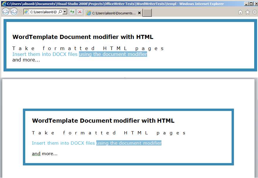
In OfficeWriter 8.0, we added the ability to embed RTF or HTML documents in Word files with WordTemplate.  The feature uses the document modifier to signify that a RTF or HTML document will be inserted. To learn more about using the document modifier, see our guide on inserting an embedded document under our WordTemplate Tutorials.

HTMLtoWord

We have also extended the feature to include DOCX files. Now you can embed other Word documents into your WordWriter templates. Continue reading What’s new in OfficeWriter 8.5

Optimizing ExcelApplication performance to reduce memory or time usage

Problem

Your program, which uses the ExcelApplication object, is using more memory than you would like or is taking too long to generate a report.

Solution

The Best Pratices with Large Reports article in our documentation discusses how to optimize for large ExcelApplication reports by reducing memory or run time. It includes, but is not limited to:

  • What to avoid when referencing cells, inserting rows or columns, and applying styles
  • Certain methods are known to be memory intensive, such as AutoFitWidth
  • Ways to improve performance by changing how and when data is imported

There are also code examples that compare inefficient code and code that was improved by the recommendations in the article. These code examples are split up into Memory Related Performance Issues and Time Related Performance Issues.

How to create a dual axis chart from bar charts

Problem

With the ExcelApplication object, it is possible to create and manipulate charts, including bar charts with series on both the primary and secondary axes. In this example, we will cover how to use OfficeWriter to create a dual axis bar chart.

Note: The ExcelApplication object is only available in OfficeWriter Enterprise Edition (EE).

Solution

This example assumes that you are familiar with creating charts with ExcelApplication. If you’re not, we recommend that you check out Charts in ExcelApplication.

Let’s start with given data in worksheet Sheet1:

The following code snippet creates a bar chart with two series from that data:

Worksheet wkst = wb.Worksheets["Sheet1"];
Anchor anchr = wkst.CreateAnchor(5, 5, 0, 0);


//Create the chart
Chart chrt = wkst.Charts.CreateChart(ChartType.Bar.Clustered, anchr);


//Set the category axis data for the chart
chrt.SeriesCollection.CategoryData = "A2:A4";


//Create a cluster bar series on the primary axis
Series series1 = chrt.SeriesCollection.CreateSeries("B2:B4", ChartType.Bar.Clustered, AxisType.Primary);


//Create a cluster bar series on the secondary axis
Series series2 = chrt.SeriesCollection.CreateSeries("C2:C4", ChartType.Bar.Clustered, AxisType.Secondary);

If you are working with an existing chart, you can set the Series.AxisType property to AxisType.Secondary.

 series2.AxisType = AxisType.Secondary 
This will produce a chart that looks like the following:

The reason why only one series appears on the chart is because of an issue with how Excel displays bar and column charts on two axes.

To get around this, you should pad your data with zeroed values which act as placeholders for the bar or column chart series. Peltier Tech has a blog post with details on how to show a Column Chart on Two Axes. These principles also apply to bar charts.

This workaround can also be applied to OfficeWriter charts.

Dual Axis Chart Workaround

1. Pad the data to include the zeroed columns.

2. Add code for the place holder series on the primary and secondary axes


//Create a cluster bar series on the primary axis
Series series1 = chrt.SeriesCollection.CreateSeries("B2:B4", ChartType.Bar.Clustered, AxisType.Primary);


//Create the zeroed placeholder series for the primary axis
Series series2_pad = chrt.SeriesCollection.CreateSeries("C2:C4", ChartType.Bar.Clustered, AxisType.Primary);


//Create the zeroed placeholder series for the secondary axis
Series series1_pad = chrt.SeriesCollection.CreateSeries("D2:D4", ChartType.Bar.Clustered, AxisType.Secondary);


//Create a cluster bar series on the secondary axis
Series series2 = chrt.SeriesCollection.CreateSeries("E2:E4", ChartType.Bar.Clustered, AxisType.Secondary);

3. Add code to hide the legend entries for the placeholder series:
//Hide the placeholder legend entries
series2_pad.ShowLegendEntry = false;
series1_pad.ShowLegendEntry = false;

The final chart should display both series correctly on the separate axes:

Note: The change in color is because there are technically 4 series in the chart and Excel’s automatic coloring reflects this.

How to format alternating color rows with ExcelApplication

Problem

A common way to display data in Excel is to alternate the background color of every other row when displaying a large table of data. With ExcelWriter there are multiple ways to accomplish this. This post covers some possible ways to apply alternating row colors with ExcelApplication.

There is another post that discusses how to do this with ExcelTemplate.

Solution

In versions of ExcelApplication prior to 6.5.1, the only way to set alternating background colors on a table was to loop over all the rows you wanted to format and set their background colors one at a time. This can take a long time for large amounts of data, and requires quite a bit of code. With the introduction of the ConditionalFormat object in ExcelWriter 6.5.1, alternating row colors in a Range with the ExcelApplication object is much simpler and faster.

The first step is to choose colors for the odd and even rows. In this example I’ll color even-numbered rows a light blue and odd-numbered rows white. You can use any colors you like, as long as they exist in the Palette or you add them yourself.

The second step is to create the ConditionalFormat object and the conditions within it. Each Condition has a comparison rule that gets set up in the constructor and a Style object that will be applied to each cell for which that rule is true. To alternate row colors we need two Conditions: one that will format the odd-numbered rows and one for the even-numbered rows.

To do this we use the FormulaEvaluation comparison type and create formulas that evaluate to true depending on the numbering of the row. The MOD() function returns the remainder left after dividing its first argument by its second, and the ROW() function returns the 1-indexed number of the current cell’s row. Thus, MOD(ROW(), 2)=1 will be true for all odd-numbered cells, and MOD(ROW(), 2)=0 will be true for odd-numbered cells.

After creating the conditions, we change the formatting of the Style objects associated with them. For this example all we’ll do is change the background color, but we could apply any formatting that can be set with through the Style object. As in the example below, we suggest that you modify the existing Condition.Style object rather than creating a new Style object and setting Condition.Style to it, as some attributes are not preserved properly with the second method.

The final step is to create the Range this formatting should be applied to and associate the ConditionalFormat with the Range. The following code illustrates these steps and produces the screenshot below.


// Create the colors we'll use on alternating rows. In Excel you can only
// use colors in the Palette, so we need to create a Palette object and use
// that to get the colors.
Palette p = wb.Palette;
Color evenColor = p.GetClosestColor(153, 204, 255);
Color oddColor = p.GetClosestColor(255, 255, 255);


// Create the conditional format and its conditions. Each condition
// has a formula that can evaluate to true or false.
ConditionalFormat oddEvenColors = wb.CreateConditionalFormat();
Condition evenRows;
evenRows = oddEvenColors.CreateCondition(Condition.Comparison.FormulaEvaluation, "=MOD(ROW(), 2)=0");
Condition oddRows; oddRows = oddEvenColors.CreateCondition(Condition.Comparison.FormulaEvaluation, "=MOD(ROW(), 2)=1");


// Change the background color for each condition. This is what will change
// for the cells where the condition is true.
evenRows.Style.BackgroundColor = evenColor;
oddRows.Style.BackgroundColor = oddColor;


// Create the range we want to format and set the formatting.
Range toFormat = ws.CreateRange("A1:F10");
toFormat.SetConditionalFormat(oddEvenColors);

Note that the conditional formatting is applied rather than set. This means that only the differences between any existing styles and the conditional formatting will take effect. For example, if some of the cells in the range had a border or had changed the font size, those changes will not be affected when we change the background color. See our documentation for more on setting and applying styles.

Modifying an existing named range with ExcelWriter

Problem

If a workbook created with Excel or ExcelWriter contains a named range, can the named range be modified (i.e. modify the areas it references)?

A customer asked about this specific scenario:

For example, when the document was first created a named range called “DataRange” was created in the workbook referencing cells A1:B9 on sheet1. The end user has been instructed to create pivots and charts based on this named range.

Then at a later date when new data is available I want to refresh the data in that spreadsheet and refresh the named range. If the number of rows of data has changed, say going from 9 records to 12, how can I update the existing named range to include the new area and thus have all the pivots/charts that were created by the end user automatically linked to the new area?

Solution

Currently there is not a way to modify the area referenced by a named range using the ExcelApplication object. There is a method Range.JoinRange that can add a new area to a named range.

In the scenario listed above, this won’t work for the customer because Excel does not let you specify a formula containing multiple areas as the data source for a pivot table. Doing so would result in a “Reference is not valid” error.

In Excel, if you insert new rows or delete rows inside an existing range, the range would be automatically adjusted; charts and pivot tables which refer to this range are automatically updated. We can follow this approach to update named ranges referenced by pivot tables.

Inserting Data Rows with ExcelApplication

  1. Open the Excel file with the ExcelApplication object.
  2. Retrieve the existing named range. using Workbook.GetNamedRange or Worksheet.GetNamedRanged.
  3. Insert enough rows to accommodate new data within the named range using Worksheet.InsertRows or Worksheet.InsertRow.
  4. Insert data into the new rows by setting Cell.Value or using Worksheet.ImportData.

Inserting Data Rows with ExcelTemplate

  1. Create ExcelWriter data markers within the existing named range (e.g. use ExcelApplication to write Cell.Value = “%%=DataSource.ColumnName”).
  2. Use ExcelTemplate to populate the data markers.

Deleting Data Rows

To delete existing rows, you can use the Worksheet.DeleteRows or Worksheet.DeleteRow method.

Customer Example

In the customer’s scenario, the new rows need to be inserted inside the named range (not at the beginning or end). Also, the pivot table must be set to “Refresh on open”, which is an option under pivot table options > data.

Error: General license key exception: No valid license key found

Problem

When trying to create an instance of the ExcelApplication or ExcelTemplate objects, the following error is returned:

General license key exception: No valid license key found.

This can happen if you are trying to use an OfficeWriter dll that is not the same version as the license key in the registry.

A common scenario where this occurs, is upgrading to a new version of OfficeWriter. When the old version of OfficeWriter is uninstalled and a new version is installed, the dlls in your projects are not automatically updated. This means that your projects may have references to the old dlls (say v4), but the license key in the registry is for the new version (v8).

Update April 4, 2013: If you are running a 32-bit application with OfficeWriter on a 64-bit operating system, you may encounter this error message, even though the license key is in the registry and matches the version of OfficeWriter being used. If you experience this issue, please contact us.

Solution

There are 2 options:

  1. Update the references in your projects to point to the new OfficeWriter dlls. (Dlls can be found under Program Files\SoftArtisans\OfficeWriter\bin).
  2. Add the license key for the old version with the License Key Manager to run both versions of OfficeWriter. For more information about running different versions of OfficeWriter side-by-side, refer to this post.

To add a license key with the License Key Manager:

  1. Locate LicenseManager.exe either from Start > Programs > SoftArtisans > OfficeWriter or from Program Files\SoftArtisans\OfficeWriter.
  2. If you are installing on Windows 7 or Windows Server 2008, right click LicenseManager.exe and select ‘Run as Administrator’. Otherwise, double-click to run the installer.
  3. Click the Add/Update Key button to add the license key.
  4. After the license key is added, you should see license keys for the old and new version registered.

ExcelWriter Error: This file does not appear to be a valid Excel 97 or later binary file

Problem

When trying to open an XLSX or XLSM file with ExcelApplication, you get the following error message:

This file does not appear to be a valid Excel 97 or later binary file. Please try opening in Excel 97 later by saving as “Microsoft Excel Workbook (*.xls)”

Solution

Support for the Office 2007/2010 file formats (XLSX, XLSM) was introduced for ExcelApplication in ExcelWriter 8. Earlier versions with throw the above exception when attempting to open an XLSX file with ExcelApplication.

Sign in to download product updates. Make sure to follow the instructions for installing a new version of the product.

ExcelWriter leaves empty space for a chart title

Problem

When using ExcelApplication to create or modify charts, there appears to be an empty space for the chart title even though one wasn’t specified or the chart title is set to an empty string.

Solution

ExcelWriter will leave space for a chart title if any of the Chart.Title properties are set; this includes setting Chart.Title.Text to an empty string. This is because ExcelWriter assumes that if Chart.Title properties are being set, then there will be a chart title.

This mimics Excel’s behavior, as chart title properties cannot be accessed or modified unless there is a non-empty chart title.

To avoid having extra space for the title, only set Chart.Title properties when Chart.Title.Text is set to a non-empty value (i.e. you intend for the chart to have a title).