Tag Archives: Excel

How to display all selected values for an SSRS multi-select parameter in an Excel report

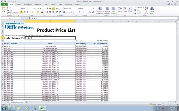
It is very common when designing reports that you may need to define a multi-select report parameter in order to give the users some filter options and generate the report based on the user-selected values. You may also want to display those selected values on the Excel report. This can easily be achieved with OfficeWriter by creating an SSRS formula that uses the required report parameter and inserting that formula into the report template through our OfficeWriter Designer add-in in Excel, as described in the following steps:

  1. Open the RDL file using the Open Report button in our add-in Continue reading How to display all selected values for an SSRS multi-select parameter in an Excel report

Super Short Tips: Working with pivot tables in VBA

Sometimes you just need to write macros for pivot tables. It’s a fact of life.

Maybe your pivot table is dynamically populated with data and you need to make some custom changes once the data is in the table, but you can only do that after the file is opened in Excel and the pivot table refreshes. Perhaps your plagued with the error that happens when you open a file with a pivot table directly from Internet Explorer. Whatever your reason, you need to write some VBA for pivot tables.

Here’s my super short list of tips for working with pivot tables in VBA:

#1 – Record a macro of yourself to get started

If you know what you want to do, but you’re not sure what the VBA code should be, record a macro of yourself doing the desired action. Not only will this give you a hint about where to start in your VBA, but you’ll also verify the exact method calls for your version of Excel and your pivot table version. All of my pivot table macros start with me performing operations in Excel and then generalizing the VBA from there.

#2 – Base your VBA on pivot fields

Pivot fields come from the column names in the data source for your pivot table. Even as the data is changing, the pivot fields remain constant because the construction and layout of the pivot table depends on the pivot fields. The fact that they remain constant can be very useful when writing VBA.

If you create macros that are based on particular pivot table items, you can’t be sure that those values will be there when the workbook is populated. For example, you want to make sure that all the groups for a particular row label are collapsed when the user first encounters the pivot table. You can manually collapse each of these groups. Problem: you create a macro that collapses groups “A”, “B”, “C”, etc separately. What if group “A” isn’t in your data set when the report is generated? Excel will throw an errror.

You can take the chance that group “A” may or may not appear in your data set, or you can create a macro that focuses on the pivot field that group “A” belongs to, rather than the individual entries.

ActiveSheet.PivotTables("PivotTable1").PivotFields("PivotField1").ShowDetail = False

This will collapse all the groups within ‘PivotField1’.

In short, avoid making macros that are dependent on specific data, because you can’t be sure that the VBA will execute without error.

#3 – VBA for pivot tables in Excel 2003 is different than in Excel 2007/2010

Excel 2003 had our best friend, the Pivot Table Wizard. Everything for the pivot table was done through a wizard menu, so the VBA in Excel 2003 follows suite. Starting in Excel 2007, Excel reworked how users interacted with pivot tables, and the Pivot Table Wizard was banished for eternity. Thus, VBA in Excel 2007/2010 is drastically different.

If you have end-users who are going to be opening a report with pivot table VBA in Excel 2003, 2007, and 2010, you’ll want to detect what version of Excel is being opened, then execute the 2003 or 2007/2010 based on this.

To determine what version of Excel the VBA is executing in, check Application.Version. This will return a string representing the version of Excel (e.g. 10.0, 12.0, 14.0 etc.)

#4 – Pivot tables have versions too

Just as there are differences between XLS and XLSX files in terms of what features can be supported, there are differences between pivot tables created in XLS files vs those created in XLSX files. What’s more, there are also differences between pivot tables created in Excel 2007 and 2010. It’s important to note what version of pivot table you’re targeting.

Luckily you can check the PivotTable.Version property to see which of the versions your pivot table is.

So there you have it – my cheat sheet for creating VBA for pivot tables.
Super Short Tips: Creating Workbooks with Excel VBA

Let’s say you want to write an Excel macro that will create a new workbook and save it to a specific location and then close the new file. This is really easy with Excel VBA:

Sub AddNewWorkbook()
     Set NewWb = Workbooks.Add
     With NewWb
          .SaveAs Filename:="C:\Path to directory\NewFile.xls"
          .Close
     End With
End Sub

You run this once and it works perfectly. You run it again and Excel tells you that “A file named ‘C:\Path to directory\NewFile.xls’ already exists in this location. Do you want to replace it?”

Well, of course you do. Why is Excel bothering you with these trivial questions?

So you want to supress the Excel alert. To do this, just set Application.DisplayAlerts to False before you save the file, and then turn it back on after you’re done:

Sub AddNewWorkbook()
     Set NewWb = Workbooks.Add
     Application.DisplayAlerts = False
     With NewWb
          .SaveAs Filename:="C:\Path to directory\NewFile.xls"
          .Close
      End With
     Application.DisplayAlerts = True
End Sub

Easy-peasy.

This technique is also handy for supressing the oh-so-lovely Do you want to save the changes you made to workbook X? alert. Microsoft has some additional tips for hiding the saving changes alert in this KB article: How to suppress “Save Changes” prompt when you close a workbook in Excel.

Stories from the WIT Trenches: Debra Dalgleish

[This is the sixth in a series of posts exploring the personal stories of real women in technology. Every woman in tech overcame at the very last statistical odds to be here; this blog series aims to find out why, and what they found along the way. If you’ve ever sought Excel-related help online or in print, chances are you’re familiar with Debra Dalgleish, one of the foremost authorities on Excel and Access development and the author of three books on pivot tables. Here, she talks staring your own home business, getting young girls aware of and excited about careers in tech and kissing correction fluid goodbye. If reading her story inspires you to share yours, please feel to email me.]

Self-employment is the dream job – most of the time. As a computer consultant, working from home, you can set your own hours, schedule meetings at convenient times, or meet with clients online. You’re the boss, so you can pass on projects that don’t appeal to you, if your workload gets too high.

If you have a young family, running your own computer-based business can give you more time with the children, while still earning an income. That’s why I got started, and now, even though the children have moved out, I wouldn’t want any other job.

My work, as an Excel and Access developer, is challenging and rewarding. My clients bring interesting projects, and push me to continue to improve my skills. In this business, there’s always something new to learn. Continue reading Stories from the WIT Trenches: Debra Dalgleish

ExcelWriter leaves empty space for a chart title

Problem

When using ExcelApplication to create or modify charts, there appears to be an empty space for the chart title even though one wasn’t specified or the chart title is set to an empty string.

Solution

ExcelWriter will leave space for a chart title if any of the Chart.Title properties are set; this includes setting Chart.Title.Text to an empty string. This is because ExcelWriter assumes that if Chart.Title properties are being set, then there will be a chart title.

This mimics Excel’s behavior, as chart title properties cannot be accessed or modified unless there is a non-empty chart title.

To avoid having extra space for the title, only set Chart.Title properties when Chart.Title.Text is set to a non-empty value (i.e. you intend for the chart to have a title).

ExcelWriter Error: Items in the array exceed 256 characters

Problem

When you specify List data validation in Excel with a sequence of comma-separated values, Excel prevents you from entering more than 255 characters, including commas. Analogously, when you create List data validation in ExcelWriter with an array of values, the CreateDataValidation method throws the exception: Items in the array exceed 256 characters, if the combined length of all of the elements in the array is longer than 255 characters. The limit is actually 255 rather than 256 as stated in the exception message. In practice, the actual limit would be lower if there are multiple elements in the array, as ExcelWriter has to insert tokens to demarcate individual values.

Solution

In order to prevent the exception, you can specify the list as a formula pointing to a range containing the desired values rather than as an array. This approach parallels Excel’s second way to create List data validation. If it’s desirable to hide the validation values, you can place the range on a non-visible area of the worksheet, or on a separate hidden worksheet.

 // Create validation object based on desired cell range 
DataValidation dv = workbook.CreateDataValidation(DataValidation.ValidationType.List, "=Sheet1!A1:A4"); 

// Alternatively, use an existing named range 
DataValidation dv2 = workbook.CreateDataValidation(DataValidation.ValidationType.List, "=ValidationRange"); 

// Set cell B1 to use validation 
worksheet.Cells["B1"].DataValidation = dv; 

For more information about creating data validations, please refer to our documentation

ExcelWriter Error: Resulting sheet would have more rows than are permitted by the Excel format

Problem

The Excel .xls binary format has a limit of 65536 rows per worksheet. If you are importing data with ExcelWriter’s ExcelTemplate object (or our SSRS renderer, which uses the ExcelTemplate object) it is possible to get an error that Excel’s row limit was exceeded even though you know you have imported much fewer than 65K rows.

This problem is usually caused by cells or formulas that already exist in the template file. When ExcelWriter populates a spreadsheet with the ExcelTemplate object, it inserts a new row for every row of data and pushes all existing rows down. If the total number of pushed down rows plus inserted rows exceeds Excel’s limit, an exception will be thrown. Then, after the data has been imported, ExcelWriter goes through the entire workbook and updates any formulas that reference the data marker cells, stretching the formulas to include all the newly inserted rows. If the cell range in a formula is stretched beyond Excel’s row limit, again an exception will be thrown.

Solution

Cells

Sometimes people take a previously populated report and turn it into a template. They may have cleared the cell values, but the template may still contain many rows of cells that are blank or contain only formatting. These rows will be pushed down when the data is imported.

The solution is to clean up the template file by actually deleting all unnecessary rows and columns rather than just clearing cell values. Also, it’s generally a good idea to set background formatting using row or column headers rather than by selecting large areas of cells.

Formulas

Formulas can be found in many parts of a workbook, including cells, charts, conditional formatting, and named ranges. Make sure that all formulas reference the minimum number of rows necessary and bear in mind that ExcelWriter will stretch certain formulas when new rows are inserted.

Hidden named ranges

It is important to know that Excel sometimes creates hidden named ranges behind the scenes for internal purposes. You won’t be able to find them through the Excel UI, but if they reference data marker cells, ExcelWriter will update them. Common cases where Excel created hidden named ranges are when the user applies an AutoFilter or AdvancedFilter to a range of cells. This occurs whether the filter is applied from the Excel UI or from a VBA macro. For this reason, check your macros carefully to make sure they are not applying any filters to unecessarily large cell ranges that include data markers. If you have any unnecessarily large hidden named ranges in your macros, you can modify them by changing the VBA code and running the macro again. If you are having trouble modifying or removing hidden named ranges, you can write some VBA code to do it. The names always end in “`_FilterDatabase”

Tip: If you have Excel 2007 or above, here is a quick way to see if you have any hidden named ranges in an .xls file without writing any VBA:

  1. In Excel, save a copy of the template file as .xlsx or .xlsm
  2. Rename to .zip and unzip the file
  3. In the subdirectory “xl”, open the file workbook..xml
  4. Look in the Section
  5. Look for defined names that end in “_FilterDatabase”. Here is an example of something you might see: <definedName name="xlnm.FilterDatabase” localSheetId=”3″ hidden=”1″> Data!$A$1:$BQ$65000
  6. If you temporarily change hidden to 0, it will show up in Excel under the named item manager.

Note: We don’t recommend permanently modifying or removing these hidden named ranges in the XML directly as that could have unexpected results.

Pitan Pivot Mage: The Mystery of the ‘Replace Content’ Message

I was working with a formatted Excel report and I needed to add a pivot table. Easy-peasy, I added my lovely little pivot table with a pivot chart. Since I would be importing the data into the pivot table later, I made sure to place the pivot chart outside of the cells that the pivot table would occupy once it was populated with data (to avoid overlap). I saved my template and went to generate my report.

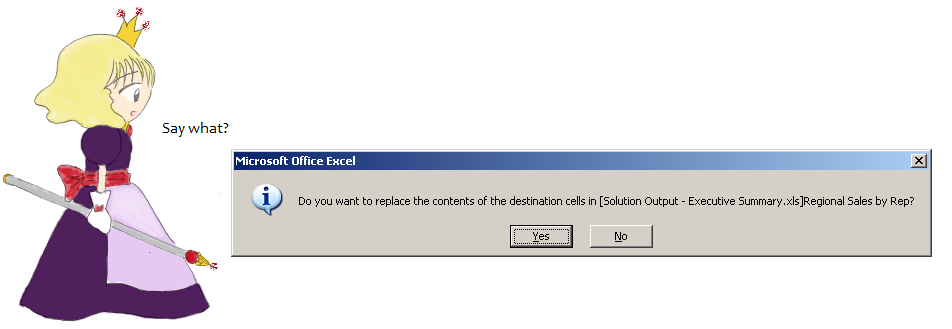
When I opened the output, I was greeted with a mysterious message from Excel:


I was baffled because I knew that nothing should overlap with the pivot table or pivot chart, even with after the data had been imported. Continue reading Pitan Pivot Mage: The Mystery of the ‘Replace Content’ Message

Trendline Label doesn’t show Equation/R-squared value

Problem

It is possible, in Excel, to add a label to a trendline of a chart that shows the Equation or the R-squared value of the trendline like in the image below:

Trendlines can also be created as objects in ExcelApplication through the Series of a Chart. The Trendline object has the properties to ShowEquation and ShowRSquaredValue.

Setting these properties to true does not seem to have any effect and the label is not shown. However, if you open, with ExcelApplication, an existing workbook which already has a Trendline label these properties will work properly. From that point on you can programmatically change the label as you like using the properties.

Solution

This issue has been resolved for charts in the OOXML file format (XLSX, XLSM) as part of implementing OOXML support for ExcelApplication in OfficeWriter v8.0.

This issue persists for the BIFF (XLS) file format. It can be worked around in the following manner:

1. Create a new chart in Excel and add a trendline.

2. Add the Equation or the R-Square: Select the trendline then right-click the trendline or choose Format>Selected Trendline from the menu.

3. Now simply open the workbook with ExcelApplication.Open, retrieve the trendline and program it any way you like (Including changing the trendline regression type or value or show/hide the Equation or R-Squared value):

Trendline trend = oSeries.Trendlines[0]; //now this will work trend.ShowEquation = true;

Error: Cannot open PivotTable source file ‘[filename[x].xls]SourceData’

Problem

When opening an Excel file containing a pivot table that was streamed to an IE client, Excel will throw the following error message:

Cannot open PivotTable source file ‘[filename[1].xls]SourceData’

This is caused by IE caching the streamed file with a temporary name containing brackets (e.g. filename[1].xlsx). Since Excel does not allow pivot table data sources to contain brackets, when the cached file is opened, the pivot tables try to refresh using the temporary file name.

Solution

There are several ways to work around this:

  • Use a non-IE browser, such as Firefox or Chrome
  • Use IE 9 or later – this appears to have been resolved in the newer versions of IE
  • Save the file to disk before opening it to avoid opening the file with a temporary name
  • Stream the file inline instead of an attachment. This will open the file in IE’s Excel plugin instead of downloading it. If you are using IE 7 or later, you will need to configure the registry on the client to use this option.
  • Add Excel macros to the report to dynamically rename the PivotTable to exclude the bracket and then refresh the PivotTable. An example of these macros is available in this blog post.

Note: This is not an issue with the OfficeWriter product. This behavior occurs anytime someone attempts to download and open an Excel workbook with a PivotTable directly from certain versions of IE.

We have made these solutions available online because our customers have found the information helpful. However, these solutions are not covered under OfficeWriter product support. If you experience issues implementing any of these solutions, we encourage you to reach out to the appropriate vendor (i.e. Mozilla for Firefox, Google for Chrome, and Microsoft for IE 9 (or later) or to configure the in-line plugin).

In particular, if you encounter difficulties with the macro solution, feel free to leave a reply on the blog post so that the author of the post can address your concerns.