BACKGOUND:
The ExcelTemplate method of creating Excel files is to design a template in Excel that contains data markers. Data markers are cell values that begin with %%= or %%=$ that specifies a database column, variable, or array to insert into the spreadsheet column. ExcelWriter does this by inserting a new row into the worksheet for each row of data being imported. This means that anything below the data marker in the template will be pushed down as the new rows of data are imported.
Data markers from the same data set can be placed next to each other, but placing data markers from different data sets side-by-side in an ExcelTemplate can cause extra rows to be inserted into the smaller data sets.
This series of posts explains how to get rid of the extra rows in output files that result from placing data markers side by side. If you’re not a current ExcelWriter user, you can download a free evaluation and follow along!
Part 2: Clearing out bad content
Part 3: Putting it altogether
Part 1: Updating Displayed Ranges from Hidden Ranges
THE PROBLEM:
Putting data markers from different data sets next to each other can be tricky, especially when the data sets are different sizes. ExcelWriter will automatically insert enough rows to accommodate the largest set of data. This means that sometimes, it ends up looking okay.
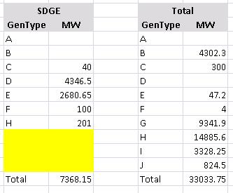
Other times, data markers like these:
Can end up being populated with extra rows like this:
A customer recently wrote in requesting a fix, since the design of his report required that the cells with the data markers be next to each other.
THE SOLUTION: COPYING THE DATA FROM ANOTHER PAGE
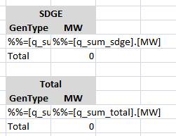
1. Create a hidden worksheet. This will be the data sheet, where the data markers will be placed one above the other (see image below).
2. Create a named range for each set of the of the data markers on the data sheet. Below are the cells in the named range ‘TOTAL’.
3. On the page where the data will be displayed, the destination sheet, create a named range that points to where the data from the data sheet should be displayed.
The named range on the destination sheet should have the same name as the corresponding named range on the data sheet, but with “_DEST” appended to the end.
For example, below is the named range ‘TOTAL_DEST’, which will display the data from named range TOTAL.
4. Use a macro to update the destination sheet based on the named ranges on the data sheet.
The data sheet’s data markers will be populated to the correct size, without additional rows, because they are above one another. Then the correct data will be displayed on the destination sheet side by side.
This is the macro to update the display range:
Sub UpdateRange(range_name As String) 'Get a reference to the source rage
Dim source_range As Range
Set source_range = ActiveWorkbook.Names(range_name).RefersToRange
'Determine the number of rows in the source range
Dim num_rows As Integer
num_rows = source_range.Rows.Count
'Define the destination range's name
Dim dest_range_name As String
dest_range_name = range_name & "_DEST"
'Declare the updated range on the side-by-side page
Dim updated_range As Range
Set updated_range = ActiveWorkbook.Names(dest_range_name).RefersToRange.Resize(num_rows, 2)
'Set the value of the updated range to be the values of the source range
updated_range.Value = source_range.Value
End Sub |
ActiveWorkbook.Names allows the user to grab named items, and requires the RefersToRange in order to return a range object. Resize() takes a number of rows and columns and returns a range of that size. It does not change the underlying range that it was called on, so the ‘updated_range’ is not the same as the destination range.
Call this on each named range on the hidden worksheet during the WorkbookOpen() event to update the table automatically when the workbook opens.
Now, this brings us to another issue…see Part 2!


 Follow