Problem
When creating workbooks with protected sheets, it is common to want to allow users to get different views of the data by sorting and filtering, without allowing them to change the data. However, while filtering works fine on locked cells, sorting does not. Even if Sort is enabled in the worksheet protection settings, if a user attempts to sort locked cells when a worksheet is protected, Excel throws the error “the cell or chart you are trying to change is protected and therefore read-only.” There is no obvious way to allow users to sort data on a protected worksheet.
Details
- Locked vs. Unlocked Cells in Excel
- About Worksheet Protection Properties
- How Protection Properties are Affected by Locked Cells
Locked VS. Unlocked Cells in Excel
The purpose of locking a cell is to prevent a user from editing the content of a cell when a worksheet is protected. This means when worksheet protection is turned off, a locked cell is no different from an unlocked cell. By default, all cells in an Excel worksheet are locked.
In order to unlock cells in Excel:
- Unprotect the sheet you are working on
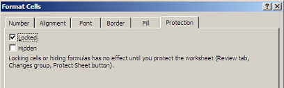
- Right-click the cell, select “Format Cells”
- Select the “Protections” tab
- Uncheck the “Locked” checkbox property
- Click “OK”
Lock Cells Dialog
It is also possible to unlock specific ranges of cells in Excel using the Allow Users to Edit Ranges feature in the Review tab. Making ranges editable for ranges of cells makes the cells behave like unlocked cells for the most part (e.g. their content is editable). However, the cell’s official locked/unlocked status does not actually change. See this Microsoft Excel article for more details about how to unlock ranges of cells.
About Worksheet Protection Properties
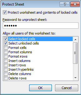
When you protect a sheet, Excel allows you to select from 15 different permissions you want to give to all viewers of the worksheet. You can allow users of the worksheet to:
- Select Locked Cells
- Select Unlocked Cells
- Format Cells
- Format Columns
- Format Rows
- Insert Columns
- Insert Rows
- Insert Hyperlinks
- Delete Columns
- Delete Rows
- Sort
- Use Autofilter
- Use PivotTable Reports
- Edit Objects
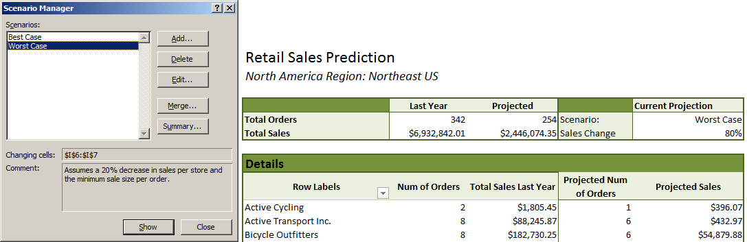
- Edit Scenarios
Protect Sheet Dialog
How Protection Properties are Affected By Locked Cells
When a cell is locked, not all worksheet protection properties operate as you’d expect. Four of the properties do not work when a cell is locked:
- AllowSort
- AllowDeleteColumns
- AllowDeleteRows
- AllowInsertHyperlinks
This is because in order to use these features the affected cell’s content must be changed. For example, using “Sort” does not just change the order of how the cells are viewed, it actually changes the values of the cells so that they are sorted. Due to this implementation of “Sort,” this worksheet protection property does not work when the cells are locked.
Solution
There are two approaches we can take to solve this issue:
Solution 1: Using “Allow Users to Edit Ranges” to Allow Locked Cell Sorting (RECOMMENDED)
This solution takes advantage of how allowing users to edit ranges makes locked cells behave like unlocked cells.
Step 1: Make cells editable so that sorting will work.
Add cells we want to sort to a range and make that range editable in “Allow Users to Edit Ranges.” This allows users to edit these cells when the worksheet is protected, even if they are locked cells.
- Select all the cells you would like the user to be able to sort, including their column headings.
- Go to the Data tab and click Filter. An arrow should appear next to each column header.
- Go to Review tab-> Allow Users to Edit Ranges
- Click “New…”
- Give the range a title.
- “Refers to Cells” should already contain the cells you want to allowing sorting on.
- If you want to allow only certain people to sort, give the range a password.
- Click “OK”
Step 2: Prevent users from editing these cells
When protecting the worksheet, uncheck “Select Locked Cells” worksheet protection property. This will prevent users from editing the cells.
- In the “Allow Users to Edit Ranges” dialog:
- Click “Protect Sheet…”
- Give the worksheet a password
- Uncheck the worksheet protection property called “Select Locked Cells”
- Check the “Sort” property and the “AutoFilter” properties
- Click “OK”
This solution allows users to use the Auto Filter arrows in the column names or the Sort buttons in the Data tab to sort data. Another benefit is that you have the option of allowing only certain users to sort by giving the range a password. Please note that this range password is separate from the password you set to protect the sheet.
Solution 2: Using Macros to Allow Locked Cell Sorting
To use a Macro to allowed the sorting of locked cells, you will need to make a macro for every sort operation you would like to allow. For example, ascending sorts and descending sorts would have to be written in separate macros. In addition, not all users have macros enabled because they are a security risk. However, the advantage of macros is that you don’t need to configure your template in any special way.
The macro we will write unprotects the sheet, selects a range called “range1,” sorts range1, and protects the sheet again:
Sub Macro1()
'
' Macro1 Macro
'
' Keyboard Shortcut: Ctrl+d
'
     //unprotect sheet
     ActiveSheet.Unprotect
     //selects range
     Application.Goto Reference:="range1"
     //clears sort
     ActiveWorkbook.Worksheets("Sheet1").Sort.SortFields.Clear
     //does descending sort, sets sort properties
     ActiveWorkbook.Worksheets("Sheet1").Sort.SortFields.Add Key:=Range("A1"), _
         SortOn:=xlSortOnValues, Order:=xlDescending, DataOption:=xlSortNormal
With ActiveWorkbook.Worksheets("Sheet1").Sort
         .SetRange Range("A1:A4")
         .Header = xlNo
         .MatchCase = False
         .Orientation = xlTopToBottom
         .SortMethod = xlPinYin
         .Apply
     End With
     //protects the work sheet again
     ActiveSheet.Protect DrawingObjects:=False, Contents:=True, Scenarios:= _
         False
 End Sub
|