Tag Archives: excelwriter

How to apply auto filters with ExcelApplication

Details

Auto filters are an Excel feature that can be applied to a column of data that allows users to select what rows of data they want visible for a given area on a worksheet.

The ability to apply auto filters programmatically with ExcelApplication in XLSX and XLSM files was added in OfficeWriter 8.3. This post covers how to add auto filters with the ExcelWriter API.

Solution

  1. Define the Area that the auto filter will be applied to.
  2. Get a handle on the AutoFilter object for the Worksheet that will have the auto filter.
  3. Set the worksheet’s AutoFilter.Area to the area that was defined earlier.

Here is the code:

Area filter_area = ws.PopulatedCells; //Returns a continuous area of all the populated cells
AutoFilter filter = ws.AutoFilter;
filter.Area = filter_area;

Here is the code in a single line:
ws.AutoFilter.Area = ws.CreateArea("A1:H1");

Additional Resources

To remove the auto filter from a worksheet, use AutoFilter.Clear():
ws.AutoFilter.Clear();
A few things to bear in mind:

  • A worksheet can only contain one area with auto filters. If you set Worksheet.AutoFilter.Area, you will overwrite any existing auto filters.
  • You must specify the entire area that you want to apply the filters to. ExcelWriter will not automatically detect blank rows and columns. We recommend Worksheet.PopulatedCells for getting a handle on all the populated cells in a worksheet.

How to hide a worksheet with ExcelApplication

Problem

A worksheet may contain proprietary data or algorithms that developers wish to hide from end-users. Different methods of hiding your data exist, but some methods are more secure than others.

Solution

An ExcelWriter workheet can be hidden by setting the Worksheet.Visibility property to Worksheet.SheetVisibility.Hidden. However, the worksheet can be un-hidden by users in Excel.

To make the worksheet more hidden, set Worksheet.Visibility to Worksheet.SheetVisibility.VeryHidden, in which case the worksheet will remain hidden unless the end-user writes a new VBA macro to unhide it.

Therefore, to keep a worksheet hidden, the developer must prevent end-users from creating new macros for the workbook as well. To do this, open the workbook’s macro editor and add a password to lock the project.

Password Protecting VBA in Excel 2007/2010

  1. Go to the Developer tab in the ribbon
  2. Go to Visual Basic
  3. Go to Tools > VBAProject Properties > Protection
  4. Check Lock project for viewing and add a password

Password Protecting VBA in Excel 2003

  1. Go to Tools > Macro > Macros
  2. Edit an existing macro
  3. In the macro editor, right-click the VBA project.
  4. Go to VBA Project Properties > Protection.
  5. Check the checkbox and add a password.

This will make it impossible for the user to look at your existing macros or to add a macro to unhide a sheet.

How to hide rows in a Pivot Table

Problem

ExcelWriter fully preserves existing pivot tables however the .NET implementation of the ExcelApplication object does not offer any support for manipulating the pivot tables. Since there is no way to programmatically hide pivot table rows with the ExcelApplication object this must be done in VBA.

Solution

In order to hide rows in your pivot table, you can include the following VBA which will execute when the user opens the spreadsheet in Excel.

Due to the sequence in which events are fired it is necessary to explicitly refresh the data in a pivot table in the Workbook_Open event instead of relying on the “Refresh on Open” Option in the pivot table options.

Disabling the option in Excel and refreshing the data in Workbook_Open() guarantees that the data has been refreshed after which you can the hide rows:

Private Sub Workbook_Open()
Worksheets(1).PivotTables("Pivot1").PivotCache.Refresh
Worksheets(1).PivotTables("Pivot1").PivotFields("Field1").PivotItems("Row1").Visible = False Worksheets(1).PivotTables("Pivot1").PivotFields("Field1").PivotItems("Row2").Visible = False
End Sub

Running VBA macros in Internet Explorer

Problem

Some VBA macros in a spreadsheet processed by ExcelWriter or WordWriter fail to execute when the file is opened in Internet Explorer. However, if the file is saved to the local filesystem and opened afterwards in Excel or Word, the macro works fine.

Solution

This issue is with MS Office and Internet Explorer, not with OfficeWriter. OfficeWriter preserves all VBA macros when processing a spreadsheet or document. However, not all VBA will execute in the Excel or Word browser plug-ins. In order to guarantee that all your macros will run in your OfficeWriter-generated files, it is recommended to use the Save option that will open the file in a separate Excel or Word window rather than in the browser.

For more information, see this article: Some Macro Commands Are Not Run in MS Internet Explorer.

Code samples

To make sure that your OfficeWriter-generated files are opened in Excel or Word instead of the browser, specify ‘false’ when using the Save method:
xlt.Save(Page.Response, "WorkbookWithMacros_out.xlsm", false); //ExcelTemplate
xla.Save(workbook, Page.Response, "WorkbookWithMacros_out.xlsm", false); //ExcelApplication
wt.Save(Page.Response, "DocWithMacros_out.docm", false); //WordTemplate
wapp.Save(document, Page.Response, "DocWithMacros_out.doc", false); //WordApplication

Basic tricks for creating ranges with formulas

Problem

A range is a group of cells in an Excel workbook that can span multiple worksheets, which is defined by an underlying formula that specifies the worksheets and cells included in the range. The formula references the worksheets and cells by name, for example: Sheet1!A5:A6 or Sheet2!C14:C27.

ExcelWriter provides the option of creating named and unnamed ranges programmatically. Named ranges will remain in the output file, but unnamed ranges are only defined in code. Both Worksheet.CreateRange() and one of the overloaded methods for Worksheet.CreateNamedRange() require a formula string.

Here are a few useful tips for pulling together the formulas for [defining ranges|http://wiki.softartisans.com/display/EW8/Areas+and+Ranges] with ExcelWriter.

Solution

The formulas that express a range in Excel use sheet names and absolute or relative cell names to reference groups of cells.

Cell Names

Cell names can either be relative (A5) or absolute ($A$5). When the cell name is relative, the cell name can update. For instance, a formula with the relative cell name A5 will update to A6 if a row is inserted above row 5. When the absolute cell name is used, the name does not update. Both can be used in the formulas for ranges.

For example, the two statements below create the same range using the ExcelApplication object:
Range cond_range = wb.CreateRange("=Sheet1!C7:O7");
Range vRange = wb.Worksheets[0].CreateRange("=Sheet1!$C$7:$O$7");

For additional ease, the Cell.Name object can be used to return the relative name of the cell:
Workbook.Worksheets[0].Cells[0, 0].Name; //Returns "A1"

Worksheet Names In Excel

Formulas that express ranges also need to specify the worksheet that the cells belong to in order to avoid ambiguity. The general format to fully specify cells with a worksheet is to preface the cells with SheetName!. For example: Sheet1!C4:C5.

If the worksheet name contains a space, the entire worksheet name needs to be surrounded by single quotation marks: ‘Sheet 2’!A5:A7.

Worksheet Names with ExcelWriter

Just like in Excel, if a worksheet name has a space in it, make sure to surround the sheet name with ‘ ‘. Not doing so will result in a failed parser error message: Unable to parse formula: irrecoverable syntax error.

Worksheet name with space:
Workbook.Worksheets[0].Name = "Sheet 1";
Range rng = WB.CreateRange("='Sheet 1'!$C$7:$O$7");

Worksheet name without space:
Workbook.Worksheets[1].Name = "Sheet2";
Range rng2 = WB.CreateRange("=Sheet2!$C$7:$O$7");

Worksheet.Name can be used to set or return the name of the worksheet:
Workbook.Worksheets[0].Name = "Sheet 1";

Including separate groups of cells in a single range:

Separate groups of cells can be included in the same range. Each continuous group of cells needs to be prefaced by SheetName! and separated by commas. For example: Sheet1!C5:C6,Sheet1!D5:D6,Sheet2!E7:E10 is made of three separate groups of continuous cells that span two worksheets.

Below is some sample code that adds cells in specified columns to a range:

int[] cols = { 2, 3, 6, 12, 14 }; //0-index column numbers to include in the range
string range_formula = "=";
foreach (int col in cols)
{
range_formula = range_formula + "Sheet1!" + wb.Worksheets[0].Cells[row - 1, col].Name + ",";
}

Modifying an existing named range with ExcelWriter

Problem

If a workbook created with Excel or ExcelWriter contains a named range, can the named range be modified (i.e. modify the areas it references)?

A customer asked about this specific scenario:

For example, when the document was first created a named range called “DataRange” was created in the workbook referencing cells A1:B9 on sheet1. The end user has been instructed to create pivots and charts based on this named range.

Then at a later date when new data is available I want to refresh the data in that spreadsheet and refresh the named range. If the number of rows of data has changed, say going from 9 records to 12, how can I update the existing named range to include the new area and thus have all the pivots/charts that were created by the end user automatically linked to the new area?

Solution

Currently there is not a way to modify the area referenced by a named range using the ExcelApplication object. There is a method Range.JoinRange that can add a new area to a named range.

In the scenario listed above, this won’t work for the customer because Excel does not let you specify a formula containing multiple areas as the data source for a pivot table. Doing so would result in a “Reference is not valid” error.

In Excel, if you insert new rows or delete rows inside an existing range, the range would be automatically adjusted; charts and pivot tables which refer to this range are automatically updated. We can follow this approach to update named ranges referenced by pivot tables.

Inserting Data Rows with ExcelApplication

  1. Open the Excel file with the ExcelApplication object.
  2. Retrieve the existing named range. using Workbook.GetNamedRange or Worksheet.GetNamedRanged.
  3. Insert enough rows to accommodate new data within the named range using Worksheet.InsertRows or Worksheet.InsertRow.
  4. Insert data into the new rows by setting Cell.Value or using Worksheet.ImportData.

Inserting Data Rows with ExcelTemplate

  1. Create ExcelWriter data markers within the existing named range (e.g. use ExcelApplication to write Cell.Value = “%%=DataSource.ColumnName”).
  2. Use ExcelTemplate to populate the data markers.

Deleting Data Rows

To delete existing rows, you can use the Worksheet.DeleteRows or Worksheet.DeleteRow method.

Customer Example

In the customer’s scenario, the new rows need to be inserted inside the named range (not at the beginning or end). Also, the pivot table must be set to “Refresh on open”, which is an option under pivot table options > data.

How to make the pie chart display larger

Problem

There is a known issue with pie charts that are created with ExcelApplication in the binary XLS file format. Pie chart display was improved in ExcelWriter 8 for the XLSX file format as part of the ExcelApplication OOXML implementation.

This post addresses how to improve the size of a pie chart in an XLS file.

Solution

There are two approaches for increasing the size of a pie chart:

Approach Before After
Increase the size of the chart while maintaining the proportions between the pie graphic and the chart frame. This requires making the chart (as a whole) larger.
Increase the size of the chart in relation to the chart frame. This requires making adjustments to the chart’s plot area.

Option 1: Increase the pie chart and maintain current proportions

If the pie chart graphic displays too small, increase the chart’s area by providing more room for it in Add method of the Charts object. The size of the pie graphic in the chart is directly related to the amount of space provided for the chart.

To provide more area for the chart, after adding the chart with the AddChart method:

  1. Make the chart wider by increasing the Chart.Width property
  2. Make the chart taller by increasing the Chart.Height property

Option 2: Change the proportion of the chart size in relation to the chart frame

Use the PlotArea‘s Height and Width properties. The values you can provide range from 1 to 4000. 4000 makes the chart take up the maximum area possible. In many cases, this value will be too large. For the area provided in the above code, 2500 is a good value for the PlotArea Width and height.

Solving the ‘double hop’ issue using Secure Store


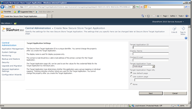
[Image via Fabian Williams]

Last week I was working on some ASP.NET web forms that generated internal reports against MS CRM using ExcelWriter and I wanted to port the application to one of our SharePoint instances. Though it seemed simple at first, I ran into a few issues. One of the issues happened to be authentication related. It was a typical ‘double hop’ problem where this SharePoint instance was using integrated Windows NTLM authentication and my code was trying to access the CRM SQL Server database. By nature, NTLM is unable to pass the credentials to the database thus producing access errors. (You can find more information on the NTLM issue and using Kerberos as a solution here.)

Since we don’t have Kerberos configured on this environment, our best solution was Secure Store. This service allows a user to authenticate with domain credentials and then use an account established in Secure Store to access the database. In our case, this was the read-only CRM account. This also enables easy to use and convenient access control using AD groups. Continue reading Solving the ‘double hop’ issue using Secure Store

Unexpected behavior of the CONTINUE modifier in version 7.1 and below

Problem

Using the CONTINUE modifier in a template to generate a report may show an unexpected behavior. Breaking down the different scenarios, we find that the behavior changes with data source type and amount of data available.

As described in our documentation, the Continue modifier enables data from a single data source to span multiple worksheets using the ExcelTemplate object. Without the modifier, if the data source for the ExcelTemplate uses a forward-only cursor, such as with a DataReader, the second worksheet with the same data marker will automatically start from the next row of data. If the data source is scrollable, however, the second worksheet with the same data marker will rewind to the first row of data. The Continue modifier tells the ExcelTemplate object to start from the next row even if the data source is scrollable. More about data markers and modifiers here.

In version 7.1 and below, the above description is accurate if there is enough data to reach the last data marker with a continue modifier before the data source has exhausted. However, if the data source gets exhausted prior to that point, the ExcelTemplate object will try to rewind the data source which may result in an exception thrown (for forward-only data sources) or duplication of data (for scrollable data sources).

Here are the two specific cases:

  1. When using a forward-only data source, the ExcelTemplate object will throw a runtime exception on the Process method: “Exhausted Data Markers” because it has encountered a new data marker but there is no more data available.
  2. When using a scrollable data source, the ExcelTemplate object will rewind the data source and will result in duplicated data on both worksheets.

Solution

Option 1: Upgrade to ExcelWriter 7.5 or later (recommended)

This issue was fixed in version 7.5 by applying more reasonable behaviors to the edge cases. With the new behavior, if the data has exhausted before reaching all data markers with a CONTINUE modifier, ExcelTemplate will not attempt to rewind the data source and will simply remove the extra data markers (similar to the behavior of the “optional” modifier).

Here is a table comparing the old and new behaviors in all scenarios:

No modifiers (CONTINUE) (OPTIONAL) (CONTINUE,OPTIONAL)
Old New Old New Old New Old New
Forward-only data source that still has data Continue Continue Continue Continue Continue Continue Continue Continue
Forward-only data source with exhausted data Exception Exception Exception Empty Exception Empty Exception Empty
Scrollable data source with that still has data Rewind Rewind Continue Continue Rewind Rewind Continue Continue
Scrollable data source with exhausted data Rewind Rewind Rewind Empty Rewind Rewind Rewind Empty

Option 2: Divide the data

If the template file cannot be modified at runtime, divide the data according to the number of sheets containing data markers with the CONTINUE modifier. This can be done by adjusting the MaxRows setting so there will be data available to the last of these data markers.

Option 3: Use ExcelApplication

Alternatively, if we have the ExcelApplication object available (included in OfficeWriter Enterprise Edition) we can modify the template to contain the correct number of sheets in the workbook. This way we can keep MaxRows a constant. It is possible to pass a template document between the application object and the template object in memory.

Error: General license key exception: No valid license key found

Problem

When trying to create an instance of the ExcelApplication or ExcelTemplate objects, the following error is returned:

General license key exception: No valid license key found.

This can happen if you are trying to use an OfficeWriter dll that is not the same version as the license key in the registry.

A common scenario where this occurs, is upgrading to a new version of OfficeWriter. When the old version of OfficeWriter is uninstalled and a new version is installed, the dlls in your projects are not automatically updated. This means that your projects may have references to the old dlls (say v4), but the license key in the registry is for the new version (v8).

Update April 4, 2013: If you are running a 32-bit application with OfficeWriter on a 64-bit operating system, you may encounter this error message, even though the license key is in the registry and matches the version of OfficeWriter being used. If you experience this issue, please contact us.

Solution

There are 2 options:

  1. Update the references in your projects to point to the new OfficeWriter dlls. (Dlls can be found under Program Files\SoftArtisans\OfficeWriter\bin).
  2. Add the license key for the old version with the License Key Manager to run both versions of OfficeWriter. For more information about running different versions of OfficeWriter side-by-side, refer to this post.

To add a license key with the License Key Manager:

  1. Locate LicenseManager.exe either from Start > Programs > SoftArtisans > OfficeWriter or from Program Files\SoftArtisans\OfficeWriter.
  2. If you are installing on Windows 7 or Windows Server 2008, right click LicenseManager.exe and select ‘Run as Administrator’. Otherwise, double-click to run the installer.
  3. Click the Add/Update Key button to add the license key.
  4. After the license key is added, you should see license keys for the old and new version registered.