All posts by Alison

Full time OfficeWriter Product Owner, part-time pivot table enthusiast.

ExcelTemplate: How to format alternating row colors

Problem

A common way to display data in Excel is to alternate the background color of every other row when displaying a large table of data. With ExcelWriter there are multiple ways to accomplish this. This post covers some possible ways to apply alternating row colors with ExcelTemplate.

There is another post that discusses how to do this with ExcelApplication.

Solution

Option 1: Format as Table in Excel 2007/2010

Starting in Excel 2007, Excel provides pre-formatted table styles which already contain alternating row or column colors. This is the easiest way to format your data with alternating row colors. Note: these table styles may not render properly in Excel 2003 or in the XLS file format.

To format an area of cells as a table:

1. Highlight the area of cells.

2. Go to Format as Table in the ribbon.

3. Select a table style from the available styles.

4. If you chose to include your table header row, make sure to check off “My table has headers” in the confirmation dialog.

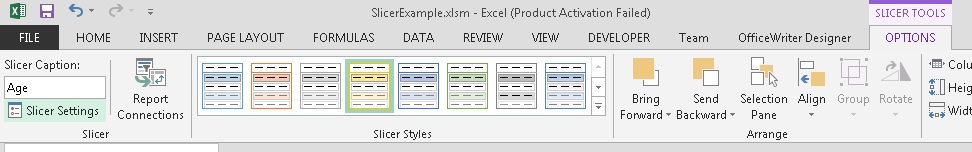
There are basic options for modifying the banding patterns:

You can also create new table styles:

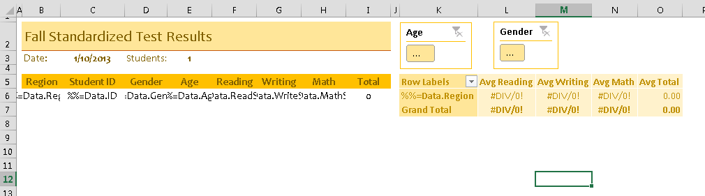
You can do this for ExcelTemplate templates:

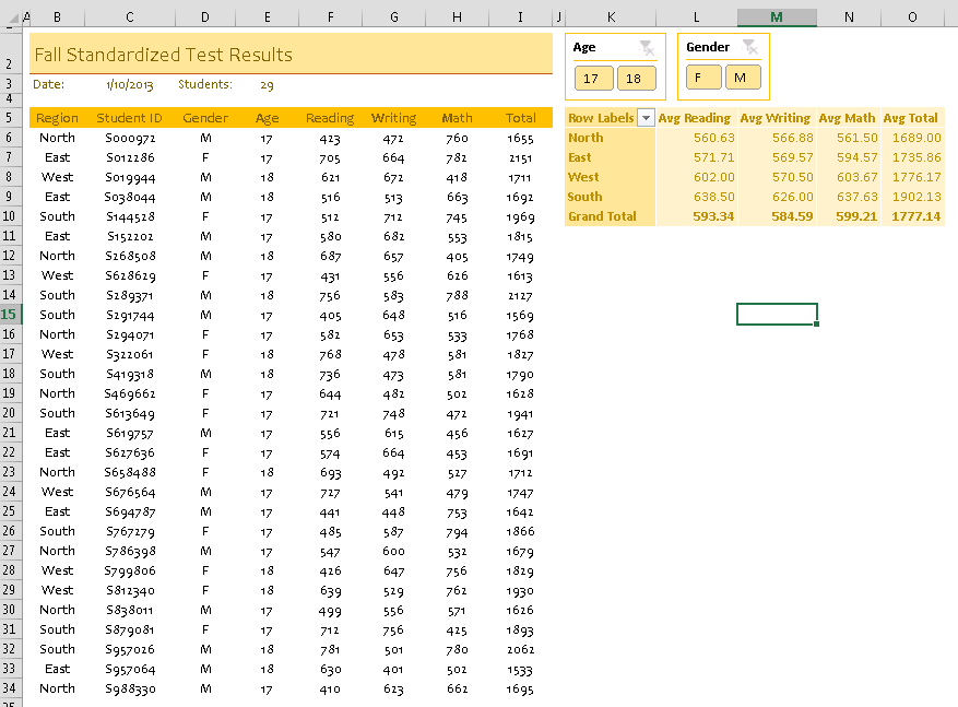
When the rows of data are inserted, the color banding will be applied:

Option 2: Use Conditional Formatting

The other approach is to use conditional formatting in the template to achieve alternating row colors. This may be more appropriate if you are not certain if your end-users will have Excel 2007/2010.

1. Create an ExcelWriter template with data markers in Excel.

2. Highlight the cells with data markers that correspond to the data you wish to display with alternating background colors.

3. From the menu, choose Format>Conditional Formatting. The formatting you define for this row will be applied to every new row that will be inserted by ExcelTemplate at runtime.

4. First define the formatting for even rows. In the “Condition1” field, choose “Formula Is” and in the formula field, type the following formula:

 =MOD(ROW(),2) = 0 

This formula uses the MOD( ) function to determine if the number of the current row (returned by the ROW( ) function) can be evenly divided by 2.

5. Click on the “format” button.

6. Click on the “patterns” tab and select a background color.

7. Now set a condition for odd rows, by clicking “ADD” and following the same steps as above but with a different formula:

 =MOD(ROW(),2) = 1 

8. Save the template and use it in your ExcelWriter application.

When ExcelTemplate imports new rows of data, the conditional formatting will also be applied to all the new rows:

How to open a report from SQL Server Reporting Services with the Application object

Problem

You want to modify your reports with the WordApplication or ExcelApplication object after they’ve been populated with data by SQL Server Reporting Services. The ExcelApplication or WordApplication object’s Open method can’t pull a report from a report server, so how do you open a SSRS report with OfficeWriter?

Solution

For simplicity and ease of reading the code examples and text in this article refer to the ExcelApplication object exclusively. However, the exact same techniques can be used with the WordApplication object. The only strict requirement for opening reports from SSRS is for the Open method to have an overload that takes a Stream argument, which both objects have.

SQL Server Reporting Services exposes a web service that lets programs access and work with the reports on the server. The web service has a number of functions for interacting with a report server and in fact is the same API that the Report Manager tool is built on top of. One of its functions will let us retrieve a fully rendered report that we can then pass to the ExcelApplication object. Once the ExcelApplication object has opened the report, it can be used as if it were any other file.

Getting a Reference to the Report Server

There are a number of different ways to access a report server to manage your reports. The MSDN documentation has detailed instructions for all the different techniques. The most powerful way, and the one that the Report Manager application uses, is to use the report server’s web service, or SOAP API. The easiest way to use the web service is to add the report server as a web reference in Visual Studio. This will allow us to make web service calls to the report server as though it were any other object in a .NET project. I’ll provide a brief overview of the steps to add a report server as a web reference; details can be found at MSDN. Continue reading How to open a report from SQL Server Reporting Services with the Application object

Workbook colors are not displayed as expected in older versions of Excel

Problem

When using ExcelWriter’s ExcelApplication object to generate a new workbook, custom colors that are assigned in code to fonts, charts, cell backgrounds, etc., display incorrectly on the client when the workbook is generated.

OR

When creating an Excel File or an Excel file to use as a template with the ExcelTemplate object using Excel 2007 and above, colors are not colors are not preserved in Excel 2003 or older.

Continue reading Workbook colors are not displayed as expected in older versions of Excel

Excel’s color palette explained

Problem

Excel’s color palette contains 56 colors, all of which can be accessed and most of which can be replaced using ExcelWriter (v6 or later). This post describes the layout of the palette and enumerate the default palette colors.

This content is most pertinent to the Excel 2003 color palette, which only has 56 colors. In Excel 2007 and later, workbooks can support millions of colors, but there is still an underlying workbook palette that has 56 colors. For more information about colors in multiple versions of Excel, we have enough post about workbook colors that are not displayed properly in older versions of Excel.

Solution

The palette is split up into a few different sections: Continue reading Excel’s color palette explained

How to create hyperlinks between cells in an Excel spreadsheet

Problem

Your application requires cells to contain hyperlinks to other cells in the same spreadsheet, but the Cell.CreateHyperlink function only makes links to URLs on the internet. This article discusses a workaround using Excel’s HYPERLINK function.

Solution

Excel has a function named hyperlink() that, with some special syntax, can create links to other cells in a spreadsheet.

Normally, the hyperlink function creates a link to a URL, much like the CreateHyperlink function. Simply passing the name of a cell to the function causes it to form a bad link; Excel will interpret it as a URL.

The solution is to enclose the name of the destination cell in quotes and preface it with a pound sign. For example, a cell with formula =HYPERLINK(“#Sheet2!C3”, “Link to C3”) will contain the text “Link to C3”, and function as a hyperlink to that cell in Sheet2. The formula can be set either by editing an Excel file directly, or through setting the Cell.Formula property in ExcelWriter.

When the user clicks on the link, Excel’s focus will move to Continue reading How to create hyperlinks between cells in an Excel spreadsheet

What’s new in OfficeWriter 8.5

Spring has sprung, bringing with it our newest release of OfficeWriter: OfficeWriter 8.5!  What’s in store for this maintenance release? Scroll down to see the latest additions our development team has been working on.

WordTemplate – Embed DOCX files into templates

In OfficeWriter 8.0, we added the ability to embed RTF or HTML documents in Word files with WordTemplate.  The feature uses the document modifier to signify that a RTF or HTML document will be inserted. To learn more about using the document modifier, see our guide on inserting an embedded document under our WordTemplate Tutorials.

HTMLtoWord

We have also extended the feature to include DOCX files. Now you can embed other Word documents into your WordWriter templates. Continue reading What’s new in OfficeWriter 8.5

5 Underutilized Excel Features To Take Advantage Of

Let’s get straight to the point, because frankly who wants to waste any more time finagling your data and reports? The following are the top 5 Excel features I use on a constant basis to get the most out of my data.

For reference, you can download the example workbook I used in this post: Top5ExcelFeatures.xlsx

#5 – What-If Analysis

WhatIfAnalysis

I actually only started using this one recently, but it’s quickly become a favorite. I’m particularly fond of the Scenario Manager function. What-If Analysis is comprised of three pieces: Scenarios, Goal Seek, and Data Tables. 

Scenarios has the ability to define a scenario that is associated with a particular set of cell values. You can define new scenarios that are tied to different cell values. When a new scenario is loaded, all of the values update. This is great for flipping between Best Case and Worst Case views of a worksheet.

WhatIfAnalysis2

The other two pieces are Goal Seek and DataTablesIn Goal Seek, Excel automatically computes and finds a calculated value based on the value of another cell, such as finding an interest rate based on a monthly payment. Data Tables allows you to hook up entire tables of values based on up to two variables.

#4 – Sparklines

Sparklines

These mini-charts were released in Excel 2010 and they provide a quick way to Continue reading 5 Underutilized Excel Features To Take Advantage Of

How to tell which Office service pack is installed

A few days ago, I installed the Office 2010 Service Pack 1 and to my dismay, I couldn’t actually tell if it had installed. The version under Program and Features hadn’t changed. There were some really complicated instructions by Microsoft for determining if SP1 had been installed, but then I stumbled across Chris Heacock’s (@chrisheacock) blog post on Verifying 2010 SP1 installations, which saved me so much time.

So here you go, a rehash of how to tell what service pack is installed in Office 2010, along with 2007 and 2003!

Office 2010

  1. Open an Office application, such as Excel or Word.
  2. Go to File.
  3. Go to Help.
  4. On the right-hand side, under Version, there should be a link to Additional Version and Copyright Information. Click that link.
  5. In the About window, you should see the full version (e.g. Microsoft Excel 2010 (14.0.6024.1000) followed by an MSO number. If you see “SP1,” then you have service pack one installed.

2010

Office 2007

  1. Open an Office application, such as Excel or Word.
  2. Go to the Windows icon.
  3. Go to Excel Options (or the equivalent for the application you’re using, such as Word Options).
  4. Go to Resources.
  5. Under Resources will be a section about Microsoft Office Excel 2007 (or Word etc.) Continue reading How to tell which Office service pack is installed

How to select slicer values with VBA

PitanHeader_short

Hello, everyone, and welcome to another edition of Pitan Pivot Mage!

Today we will cover how to select slicer values with VBA. This is especially useful if you have a report generated by OfficeWriter’s ExcelTemplate model and you can’t select the slicer values in the template file.

Intro

Let’s start out with an ExcelWriter report template. It has some data off to the side and a PivotTable that summarizes the test scores with averages. There are two slicers for filtering on age and gender.

Template

When it’s populated with data, all of the values in the slicers are automatically selected, so the default is a full view of the data.

RenderedReport

Writing the Macros

Whenever I need to write a PivotTable macro, I always start by recording myself performing the action I want and then generalize the code later. In this case, I want to select only “M” and “17” in my slicers for 17-year-old male students.

My first pass gives me some useful information:

RawMacro

The first thing I notice is the slicer name “Slicer_Age1” and “Slicer_Gender1”. This is the name for the slicer for formulas and VBA. To find the name of your slicer, select the slicer and go to slicer settings. This is on the left, under slicer tools:

SlicerTools_Settings

The slicer tool dialog lists the name of the slicer, but also the Name to use in formulas. This is the programmatic name for the slicer that we’ll use in the macro.

Slicer_Programmatic_Age

Then I was able to generalize the macro to take a slicer name, value, and whether it should be selected or deselected:


'Selects or deselects a value (slicerVal) in a slicer (slicerName)
Sub SelectSlicerValue(ByVal slicerName As String,
ByVal slicerVal As String, ByVal isSelected As Boolean)
ActiveWorkbook.SlicerCaches(slicerName).SlicerItems(slicerVal).Selected = isSelected
End Sub

To make things easier for myself, I  created a subroutine that would select 17 and “M,” while deselecting 18 and “F.”

'Selects slicer values to display only data for 17-year-old male students
Sub SelectMale17Profile()
SelectSlicerValue "Slicer_Age1", "17", True
SelectSlicerValue "Slicer_Age1", "18", False
SelectSlicerValue "Slicer_Gender1", "M", True
SelectSlicerValue "Slicer_Gender1", "F", False
End Sub

Calling the Macros

To make sure that the macro runs when the workbook is opened, I called the subroutine in the Workbook_Open() code.


Private Sub Workbook_Open()
SelectMale17Profile
End Sub

Handling the PivotTable refresh

As outlined in our tutorial for how to use PivotTables with ExcelTemplate reports, the PivotTable needs to refresh in order for the imported data to display; the easiest way to do this is to set ‘Refresh on Open’ under PivotTable Data Properties. This poses a problem because macros in Workbook_Open() execute before the the PivotTable refresh and the slicer macros will be unable to find the values to select. This results in a run-time error.

To avoid this problem, I wrote a quick macro that refreshes the PivotTable:

'Refreshes the PivotTable as a replacement for the 'refresh on open' property
Sub PivotTableRefresh(ByVal pivotTableSheet As String, ByVal pivotTableName As String)
ActiveWorkbook.Sheets(pivotTableSheet).PivotTables(pivotTableName).PivotCache.Refresh
End Sub

And added it before the slicer code in Workbook_Open().

Private Sub Workbook_Open()
'Refresh the PivotTable with a macro because it may not refresh first
PivotTableRefresh "Template", "PivotTable1"
'Select the desired slicer values
SelectMale17Profile
End Sub

There you go!

SelectedProfile

Downloads

A copy of the template file with the macros, a sample output file, and the code used to populate the template file are available for download here as a zip file.

Getting started:

Learn more about ExcelTemplate or try it out in a free trial of OfficeWriter today.

    
 OR