Problem

Excel’s “Move and Size with Cells” option allows you to automatically re-size charts if the cells that contain the chart are added or re-sized.

With ExcelWriter, when the “Move and Size with Cells” option is selected in Excel, charts are not re-sized based on rows that are added from data being imported into data markers using the ExcelTemplate object (or OfficeWriter’s SSRS integration). Charts are re-sized if rows are added explicitly using Worksheet.InsertRow.

Example 

The pictures below show a file that has “Move and Size with Cells” option selected, before and after it has been processed by ExcelWriter.

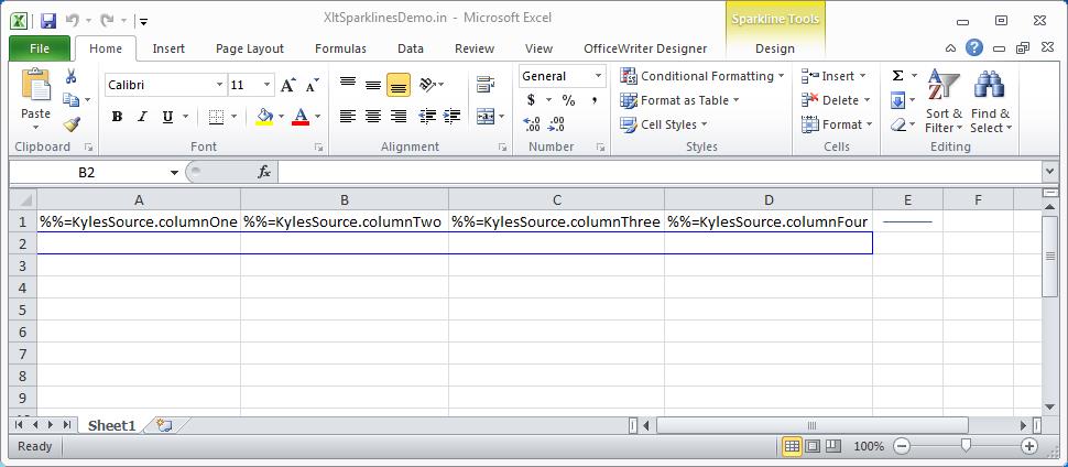
Template

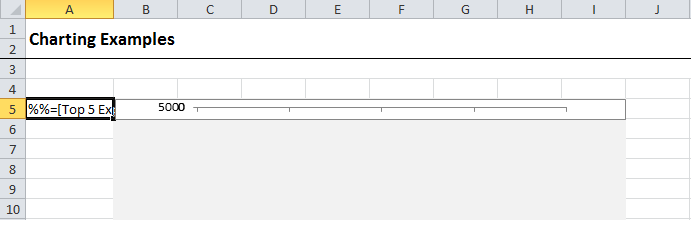
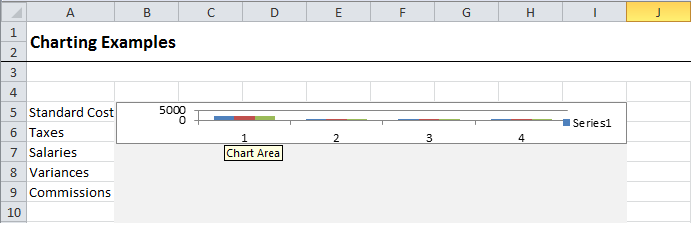
Incorrect output – Note that the chart remained the same size as before the data was imported.

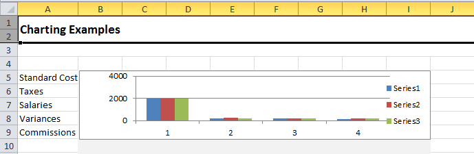
The correct output should look like the following:

Solutions

Re-sizing Excel charts to match a data set can be done programmatically with ExcelApplication or with a VBA macro. Both solutions require a named range containing the data whose height you wish to match.

Create a named range

In order to determine which data to match the size of the charts to, we will need to create a named range in your template. In the example above, a named range, called “Chart_Range” was created in cell A5. ExcelWriter will automatically expand the named range to contain all of the data imported into the data marker. Named ranges can be accessed programmatically using ExcelWriter.

Solution 1 – Use ExcelApplication

The ExcelApplication API has all the functions necessary to re-size your chart. This method assumes that you have created a named range in your template and then populated the template with data using ExcelTemplate’s Process method. Once Process is called, the named range would will expand to match the size of the imported data. In order to re-size the charts we will use ExcelApplication to determine the height of the named range by getting the heights of all the rows in the range. Then we will set the height of the chart to match. The following steps will show you how:

1) Pass the processed Template to ExcelApplication

Once our template contains data, it can be passed to ExcelApplication to be formatted. This can be done with ExcelApplication.Open.

ExcelApplicaton xla = new ExcelApplication();
Workbook wb = xla.Open(xlTemplate);
//locate the correct worksheet
Worksheet ws = wb.Worksheets["ChartingExample"];

2) Get the Named Range

Now we must locate the named range we created earlier:

//Get the named range
Range chartData = wb.GetNamedRange("Chart_Range");

3) Get the Area with the populated cells from the Named Range

In order to determine the heights of the rows we create an Area object.  The Area can be obtained through the named range.

//Get the area
Area dataArea = chartData.Areas[0].PopulatedCells;

4) Get the height of the Area by looping through all the rows

Now we can determine how tall the area is by getting the heights of all the rows in the area. Row heights are returned in points.

//A variable to keep track of the heights
double rowHeights = 0;

//loop through the rows
for (int i = 0; i < area.RowCount; i++)
{
     rowHeights = rowHeights + dataArea.getRowHeight(i);
}

5) Access and re-size the chart

Next, we need to get a handle on our chart.  The call below gets the first chart in the worksheet.  Once we have the chart we can easily set the height of the chart in points.

//Create a Charts object
Charts charts = ws.Charts;
Chart chartToResize = ws.Charts[0];

//re-size the chart
chartToResize.Height = rowHeights;

Now when you save and open your workbook, you chart will have the same height as the data in the range.

Solution 2 – Use a VBA macro

Using a VBA macro in your Excel template spreadsheet you can automatically re-size the charts upon opening the file.  The msdn documentation contains more general information about creating macros.

Note: Excel files containing macros must be saved as .xlsm files and may not work with very high security settings.

The following steps will walk you through this process:

1) Write the macro

The macro below will re-size the first chart in the worksheet.

The code is located in the auto_open method so that it will be run when the file is opened.

Sub auto_open()
' Method to change the size of the chart based on size of data in column
    Dim r As Range
    Set r = Sheet1.Range("Chart_Range")

    'Changes the height of the first chart to match the range height
    Sheet1.ChartObjects(0).Height = r.Height + 50

End Sub

2) Save your template and process with ExcelWriter

Your output should now have the same height as the data in the range.

For more information about charts in ExcelWriter see our documentation on Charts in ExcelApplication.

Follow

Related posts: